At Lossfunk, I’m working on self-driving intelligence, with a focus on reasoning and hierarchical agents. Reinforcement learning and world models are my broader focus; this post covers the symbolic reference policy and environment I’m building for that work. I started with a question: could Astra write a driving policy that I could inspect and run without calling the model at every frame?
I used Astra to write the Python policy, then ran it locally in CARLA. Every 50 ms, it reads the simulator state, picks a target speed and sends steering, throttle and brake commands. Astra is out of the loop once the car starts moving.
I wanted to be able to explain a brake command by following the code: which actor was in the way, how much clearance it left, and which rule reduced the target speed. That led to the symbolic layer.
In this article
The environment I’m building
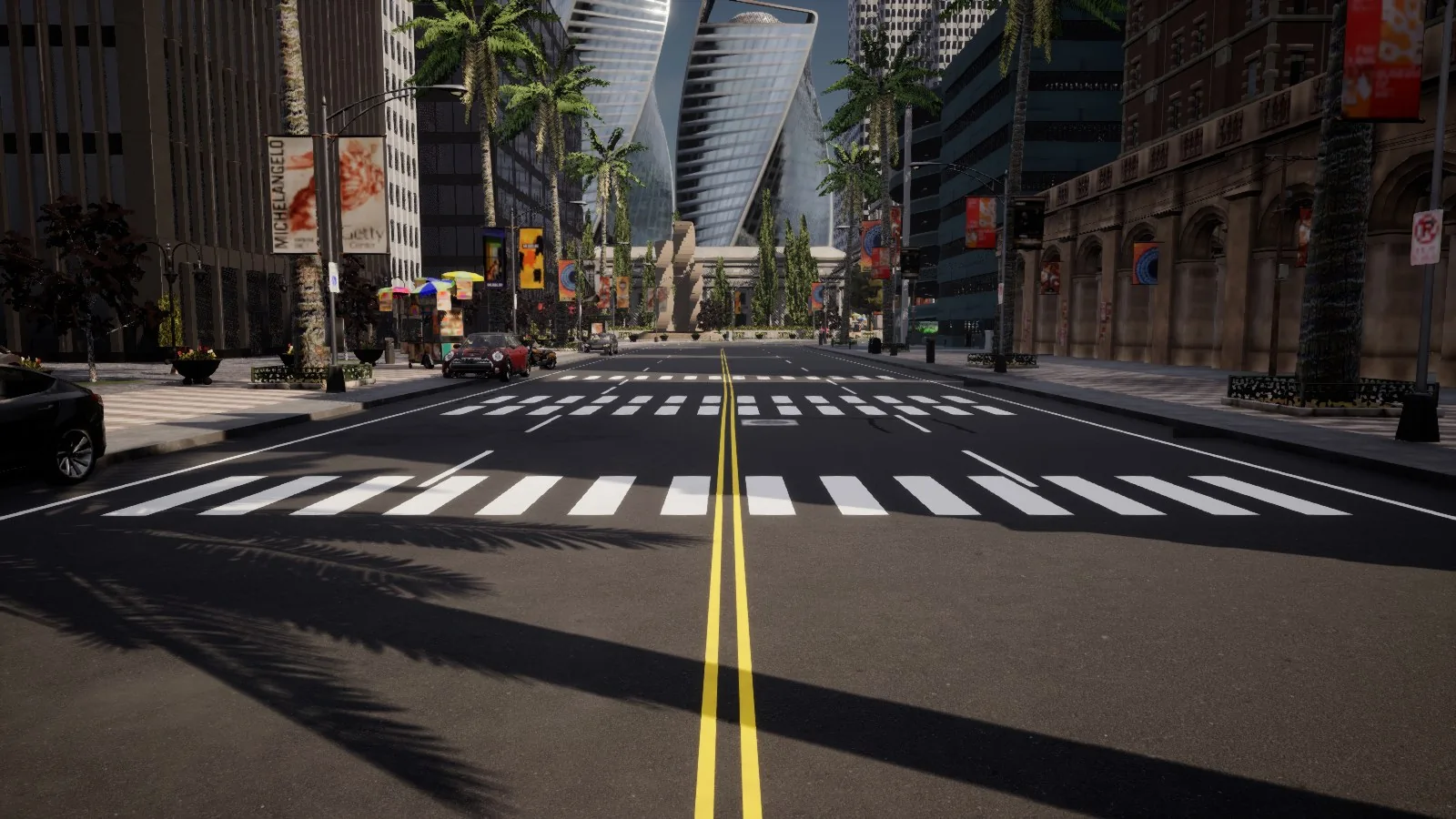
I’m also building a larger CARLA map for the next experiments. It has city streets, elevated connectors and rural roads. Here are three sections from a road-inspection drive.
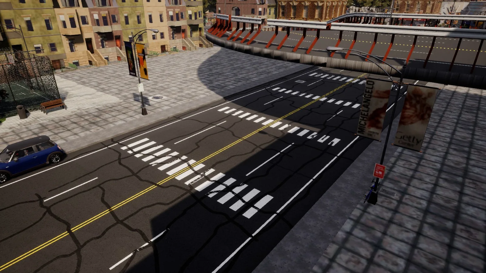
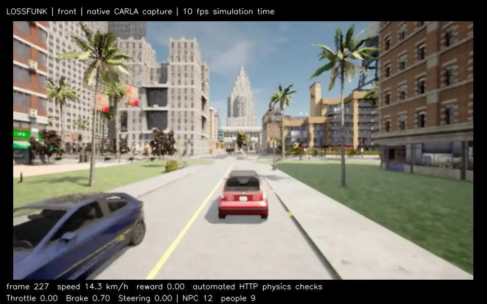
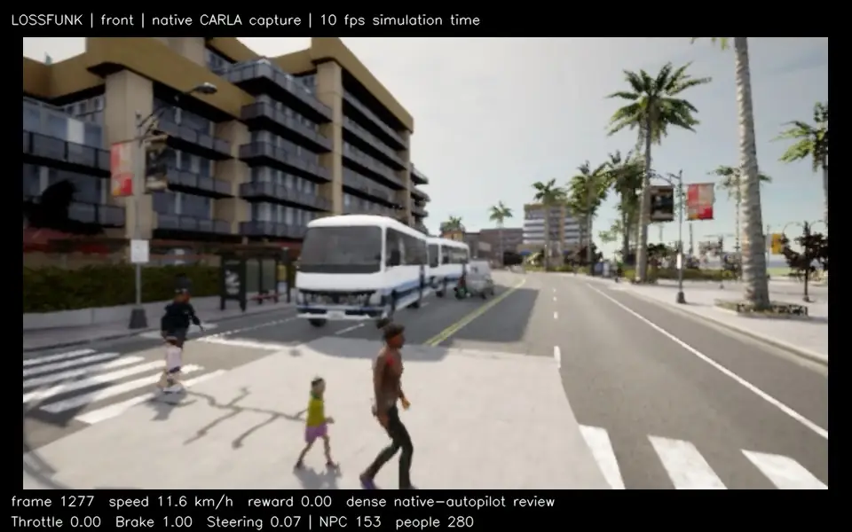
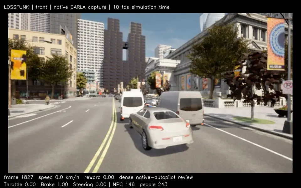
City views from the local recordings. The overlays identify the controller used in each run.
The four Town01 policy runs use Astra’s Python code. The larger-map clips show the environment and engineering tests, using their own test controllers.
What the policy sees
CARLA is the simulator. Its adapter provides the controlled vehicle’s speed, speed limit, route points, nearby actors and their dimensions and velocities, signal state, stop-line distance, and remaining destination distance. The observation interval is Δt = 0.05 s.
The adapter expresses the scene relative to the ego vehicle: forward and right rotate with the car. Town labels and road IDs do not select a driving rule. Actor IDs identify which object supports an explanation, while measured geometry determines the response.
That is a useful abstraction, but it is also privileged information. The controller receives accurate actor state from CARLA and a route from navigation. It does not identify pedestrians in RGB images or discover a destination route. The cameras in the recordings let us watch the experiment; they are not its control input.
Three jobs in one synchronous loop
- System 2 / decide
- Construct grounded facts and combine their numerical constraints into a current subgoal and target speed.
- System 1 / control
- Track the route with pure pursuit and convert target-speed error into bounded throttle and braking.
- System M / adapt
- Learn a small correction to the vehicle’s acceleration model and report unexpected dynamics.
- 01 / ObserveCurrent CARLA state
- 02 / UpdateScore the previous transition; learn
- 03 / Ground + decideFacts → constraints → target
- 04 / ControlSteer, throttle, brake
- 05 / AdvancePredict next speed; apply action; tick
These names describe roles in ordinary executable code. System 2 does not make a fresh language-model call or search over symbolic programs on each tick.
Give “ahead” a geometric meaning
An object can be visible ahead without blocking the intended route. The grounder projects each actor onto the route polyline and tests its lateral occupancy against the driving corridor. Actor width matters: a truck can intrude into the corridor even when its centre lies outside it.
For a relevant actor, the program derives front clearance using along-route position and actor length. It also records forward velocity and, when the ego is closing, a time-to-collision estimate. A separate constant-velocity forecast checks possible route conflicts over four seconds.
predicate: vehicle_ahead
actor:     current truck binding
clearance: 20.0 m
speed:     0.0 m/s
closing:   8.0 m/s
ttc:       2.5 s
This is an illustrative fact, not an extracted trace row. Each field has a physical interpretation. I can inspect the actor that was bound, the corridor test that made it relevant, and the measurements passed to the planner.
The same procedure grounds pedestrians, obstacles, crossing conflicts and stop signals. A pedestrian entering the corridor introduces a yielding constraint. As it approaches, the permitted speed decreases; a stop or emergency condition can drive that target to zero. When the route is clear again, that constraint disappears and the remaining limits determine the new target.
Reuse happens through new bindings
A different truck can instantiate the same predicate with a different gap and velocity. Translating and rotating an otherwise equivalent scene together preserves its ego-relative relations. Renaming actor IDs preserves the control output. These are useful properties of the written program, with regression coverage in the implementation.
They are narrower than learned generalization. The system is reusing existing grounding and control rules. It is not learning new symbolic programs or proving that a visual representation will discover the same relations.
Follow a fact all the way to the brake
The planner gives each applicable fact a speed constraint. A common form is a stopping envelope:
Here d is available distance, m is a reserved margin, and ab is assumed braking deceleration. The values differ by relation: the signal rule uses 2.5 m/s² and a 2.5 m margin; pedestrian and crossing constraints use 3 m/s² and 4 m. These are controller assumptions, not measured safety guarantees.
Following a lead vehicle adds a speed-dependent gap. With ego speed v, lead speed va and front clearance d:
va + √(6 max(0, d − 3))]
Distances are in metres and speeds in metres per second; the coefficients carry the matching units. On a valid route, the ordinary target is the smallest of the speed limit, curvature cap and clamped fact constraints. Emergency checks can force a stop. Dynamics surprise can reduce the target further.
An analytic 50 ms cycle
Take a straight route, an ego speed of 8 m/s and a stationary vehicle with 20 m of front clearance. Assume the destination is distant, other limits are looser, and no emergency or surprise override applies.
- Ground. The actor occupies the route corridor. Its clearance is 20 m, lead speed is zero, and closing TTC is 20/8 = 2.5 s.
- Constrain. Desired gap is 4 + 1.5 × 8 = 16 m. The gap term gives 0.5 × (20 − 16) = 2 m/s; the second envelope is looser. The selected subgoal is
follow, with target u = 2 m/s. - Control. Speed error e = u − v = −6 m/s. Ordinary braking B = min(1, max(0, −0.25e)) saturates at 1, and throttle is zero. Pure pursuit independently computes steering from the route.
- Predict and execute. With an initial zero residual, the acceleration prior predicts −7.96 m/s² and a next speed of 7.602 m/s. CARLA applies the command for 0.05 s. Its next observed speed is a measurement, not something this calculation guarantees.
- Repeat. On the next tick, score the observed transition, update the dynamics learner, and recompute the facts and controls from the new observation.
Try the following rule with a different gap
This calculator applies the straight-route rule above. It assumes a distant goal, an 8.33 m/s speed cap, no surprise, and no additional hazards. It includes the vehicle emergency check. It is an explanation of the formula, not a driving simulator.
Desired gap 16.0 m · target 2.00 m/s · throttle 0.00 · brake 1.00 · ordinary following
The plan also carries readable steps such as maintain_clearance and resume_when_clear. Those labels explain the policy; no stored program counter advances through them. The actual decision is recalculated every tick.
Two kinds of surprise
System M learns how ego speed responds to control. It begins with a simple physical prior and adds a bounded neural residual:
The residual is a 6 → 16 → 1 tanh network, bounded to ±2 m/s². Its features are speed, throttle, brake, steering and speed-control products. It sees neither images nor a representation of nearby traffic.
At the next observation, the learner compares the measured acceleration, clipped to its implemented learning range, with its prediction. The normalized error score is:
The variance is taken before its update. If S exceeds 4.5, the valid-route planner scales its freshly computed target by 0.7. This is a conservative heuristic for dynamics mismatch, rather than a calibrated probability of danger.
A truck appearing can change the grounded facts even when the vehicle responds exactly as predicted. Conversely, unexpectedly weak braking can raise the dynamics error without any new actor appearing. Treating both as one kind of “novelty” would hide what the current model actually measures.
The policy therefore has memory: learned weights, error variance and the preceding speed/action pair. The same current geometry need not produce the same command if the retained dynamics history differs. Replay needs that history or a matching reset state.
Five controlled scenarios
The documented evaluation covers lane following, a blocked lane, a pedestrian crossing, a red signal changing to green, and a newly appearing truck in Town02 with a different ego vehicle. Hazards are scripted and routes are supplied.
On a narrow screen, scroll the table horizontally to read all three columns.
| Check | Reported outcome | What it supports |
|---|---|---|
| Original scenario episodes | 5 / 5 passed | Completion under the five designed conditions |
| Nominal route distance | 499.45 m | The small scale of the evaluation |
| Collision / lane-invasion callbacks | 0 / 0 | No recorded events of these types in those runs |
| Regression suite | 16 tests passed | Specified implementation properties |
| Decision replay | 3,812 / 3,812 rows | Agreement within 10⁻¹⁰ absolute tolerance across nine traces |
The nine traces comprise five original episodes and four camera reruns of existing setups. The reruns add repeatability evidence, not four independent scenario families. Replay agreement checks implementation consistency; it does not establish physical safety or learned generalization.
The aggregate results above come from the implementation repository. I could recover the code and four recordings, but not the original trace files, so I have not recomputed those totals.
Watch the other recorded behaviours
Each clip plays at its original speed, with the same one-tick HUD offset as the blocked-lane clip. All are Town01 camera reruns. Town02 completed in a state-only run; camera capture crashed in that configuration, so there is no Town02 video here.
What I haven’t tested yet
Five short episodes cannot establish a general collision rate. Exact simulator geometry removes perception error, occlusion and uncertainty from the input problem. The current policy waits behind obstructions; it does not demonstrate overtaking, lane changes, complex intersection negotiation or dense mixed-traffic competence.
Simulation frequency also needs careful interpretation. A 50 ms simulation step establishes the control cadence used in the experiment. Deployment latency, end-to-end sensor processing and performance on constrained hardware require separate measurements.
The simulator exposed engineering failures too. Progress measured against the nearest waypoint could oscillate; continuous projection onto route segments corrected that adapter behaviour. An in-process town reload crashed, so the Town02 evaluation used a fresh server. Those fixes belong to the evidence record alongside the successful runs.
The road is part of the experiment
A control policy can be readable while the world it acts in is misleading. A painted lane may sit above the road mesh. A barrier can look connected but leave a collision gap. A material that looks wet may still behave like dry asphalt. Those differences matter when braking and contact are the quantities being evaluated.
Alongside the Astra policy work, I have been developing the more detailed Lossfunk environment: connected urban roads, elevated sections, rural edges, traffic and pedestrians. CARLA provides the runtime; Unreal Engine handles the scene and assets; OpenDRIVE supplies road and lane semantics. The environment work is ongoing.
Geometry has to survive contact
I check repairs through separate stages: geometric measurements, native collision queries, matched views, save-and-reload checks, then regional driving with cars, buses or trucks. A passing visual check cannot stand in for vehicle clearance, and a local vehicle pass does not certify the whole map.
This has exposed gaps between road and footway endpoints, stepped curbs, discontinuous barrier profiles and mismatched surface markings. Some individual junctions have passed targeted vehicle checks. Other barrier, shoulder and terrain joins remain unfinished. The broader map has not yet passed full-network physical acceptance.
These local road checks illustrate the environment-engineering work. They use the test controllers recorded for those checks, rather than the Astra symbolic policy. The short excerpts do not establish whole-map acceptance.
Bumps and potholes
I also tested vehicle response on two rough-road branches. These clips show the bump and pothole trials, from behind the car. The targeted body and wheel-diagnostic checks passed; tire contact and load still need calibration.
Surface appearance and surface response
I am also building a surface layer for dry, dirt and wet conditions. Its material-response code supports smooth transitions between configured regions rather than abrupt parameter changes. The water model tracks movement between connected cells, with conservation and numerical-stability checks.
One stress test was useful: a donor-limited water update conserved mass but still oscillated between equal-height cells. Conservation alone was too weak a check. A network-wide stability bound and bounded update work address that numerical case, with regressions for network shape, unequal cell areas and update order.
The surface, adapter, control and audit suites passed 62 unit tests. The new water/material features are still disabled in driving. Per-wheel contact, wet braking, paved-to-dirt blending and hydroplaning remain unfinished.
More environment recordings
Checking the braking assumptions
The symbolic policy’s stopping envelopes assume braking strengths. The environment determines whether those assumptions hold. My next step is to measure that connection under controlled changes in vehicle response and surface conditions, with the observation and timing contract held fixed.
The policy and the environment meet at the braking assumptions. I need measured vehicle response before I can trust the stopping envelopes on a new surface.
What I’m trying next
I now have a reference policy I can inspect. When a learned controller behaves differently, I can compare its action with the grounded facts and speed constraint, rather than only checking whether it reached the destination.
My next direction is to replace privileged state with uncertain estimates while keeping this chain available for inspection. A simple front-camera baseline comes first, with a fixed information contract and measured latency. Then change one factor at a time: actor combinations, routes, vehicle response or visibility. Extra views should answer a demonstrated field-of-view failure.
I also want to study whether fast learned policies and slower reasoning can share grounded representations. A symbolic expert supplies one checkable reference for that work. The open question is whether a learned representation preserves the relations that matter when the context changes—and whether its predicted futures can improve action selection. The current dynamics residual does not yet perform that search.
Sources and implementation
The implementation and original recordings are public. Srinitish Srinivasan’s companion post explains the grounding and rule reuse in more detail.
- Public implementation, evaluation description and recordings
- Planner: following constraints, stopping envelopes and emergency overrides
- Policy: step order, steering and longitudinal feedback
- Dynamics learner: residual model and surprise score
- CARLA documentation: synchronous mode and simulation timestep
- Coulter, 1992: Implementation of the Pure Pursuit Path Tracking Algorithm
Policy results and environment tests are separate runs. The water and material-response code still needs driving calibration.