Role Overview
We exist at the intersection of rigorous mathematics and unbounded curiosity. Erdős AI Lab is a student-founded research collective devoted to advancing the frontier of artificial intelligence - from continual learning and world models to brain-computer interfaces and neuromorphic computing. The lab is funded and trusted by Entrepreneurs First (EF) and incubated at IIT Bombay. We believe the next decade of AI will not be won by scale alone, but by ideas. Sharp, original, uncompromising ideas. That is what Erdős is built for.
Our current work centres on Knowledge Distillation (KD) and teacher-student model research - making large, powerful models more efficient and accessible by transferring their knowledge to smaller, faster student networks without significant loss in performance. We develop new KD algorithms, analyse the transfer of representations, and build robust pipelines for training and evaluating teacher-student architectures at scale.
Key Projects & Contributions
-
Novel KD AlgorithmsDesigned and benchmarked new knowledge distillation strategies for transformer and vision models, improving student model accuracy and generalization.
-
Teacher-Student Model PipelinesBuilt scalable pipelines for training, evaluation, and ablation of teacher-student architectures, supporting both supervised and self-supervised learning setups.
-
Representation Transfer AnalysisAnalyzed how knowledge is transferred at different layers and modalities, leading to insights on what makes distillation effective for various tasks.
-
Efficient DeploymentEnabled real-world deployment of compact student models on edge devices and in production, maintaining high accuracy and low latency.
Publications & Research
Geometric Limits of Knowledge Distillation: A Minimum-Width Theorem via Superposition Theory
Nilesh Sarkar et al. | arXiv Preprint
Abstract
Knowledge distillation (KD) compresses large teacher models into smaller, deployable student networks. However, student performance consistently saturates at a loss floor that persists regardless of training method, objective function, or hyperparameter tuning. We prove that this floor is geometric in origin, not an artefact of optimisation.
Core Insight: Superposition Creates Hard Limits
Modern neural networks pack far more learned features into their hidden layers than they have dimensions - a phenomenon called superposition. When a teacher with hidden width dT learns N > dT features by encoding them as near-orthogonal directions, a student with width dS < dT can faithfully capture at most dS × g(α) of those features, where g(α) is a geometric packing function determined by the interference tolerance α. Features beyond this capacity are irrecoverably lost, setting a hard floor on distillation fidelity.
The Minimum-Width Theorem
We formalise this as the Minimum-Width Theorem: for a student to achieve loss within ε of the teacher, it must have hidden width at least dmin = N / g(α(ε)). Below this width, no amount of training - longer schedules, better objectives, curriculum strategies - can close the gap. The bound is tight: we construct matching lower-bound examples using sparse-autoencoder (SAE) feature dictionaries extracted from trained transformers.
Experimental Validation
We validate the theory on transformer language models by training SAEs to extract superposed feature dictionaries at each layer. Experiments measure alive-neuron counts, L0 sparsity, feature importance distributions, and per-layer capacity utilisation. The observed loss floors align quantitatively with the geometric predictions, confirming that architecture width - not training recipe - is the binding constraint on distillation quality.
Practical Implications
This research shifts the focus of model compression from "how to train" to "how to design." By estimating a teacher's superposition ratio ($N/d_T$) using Sparse Autoencoders (SAEs), we can determine the smallest viable student architecture ($d_{min}$) before beginning compute-intensive training. This provides a diagnostic tool to visualize exactly which features are "lost" during distillation, bridging hardware efficiency with model transparency.
- Architecture Benchmarking: If a student's width falls below $d_{min}$, further training compute is mathematically wasted.
- Feature Prioritization: When width is constrained, we can use SAE importance distributions to ensure high-value features are preserved.
- Interpretability Link: SAE-based feature extraction diagnoses capacity limits and reveals the specific representational collapse of the student.
Mathematical Framework: The Minimum Width Theorem
For a student model to achieve a loss within $\epsilon$ of its teacher, it must possess a minimum hidden width:
$d_{min} = \frac{N}{g(\alpha(\epsilon))}$
Where $N$ is the number of features in superposition and $g(\alpha)$ is the geometric packing function. Below this width, the student undergoes catastrophic representational collapse.
Key Experimental Results
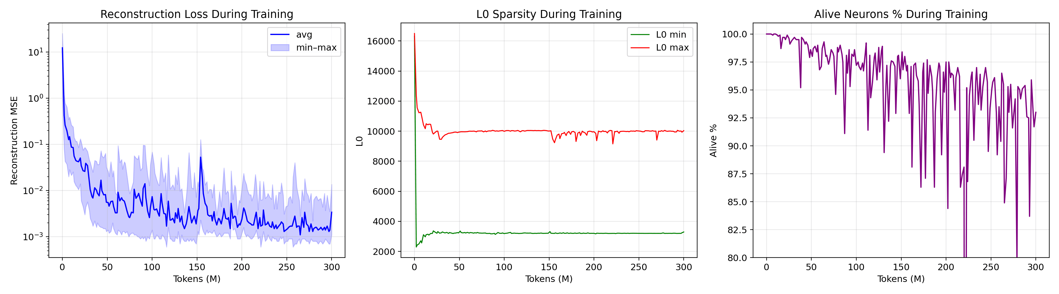
Reconstruction MSE, the L1 sparsity penalty, and the combined loss across all 24 SAE layers over 300 M training tokens. With L1 held loose at 3e-4 you get the densest activations (avg L0 around 6,184) and the best reconstruction. Each line is a layer, so the smooth simultaneous declines confirm no layer blew up.
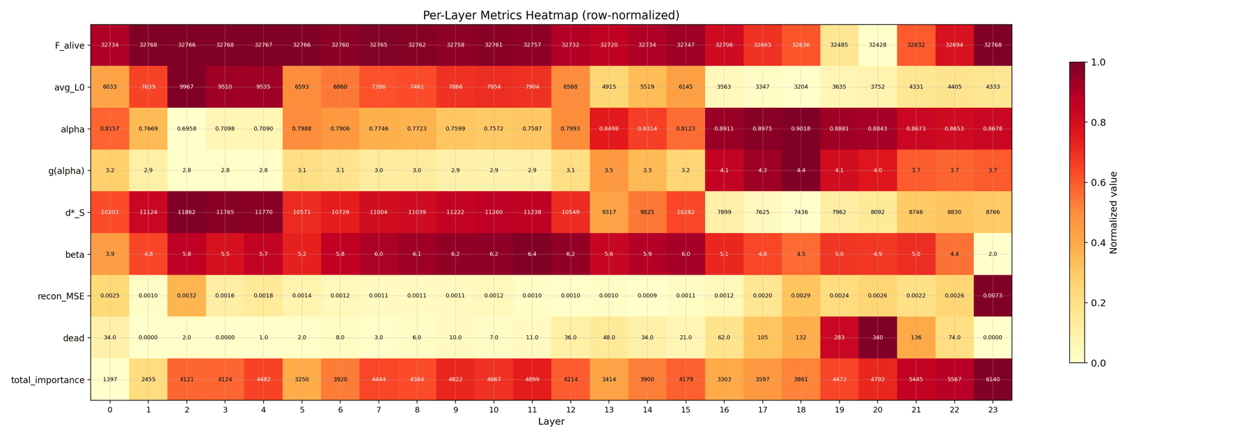
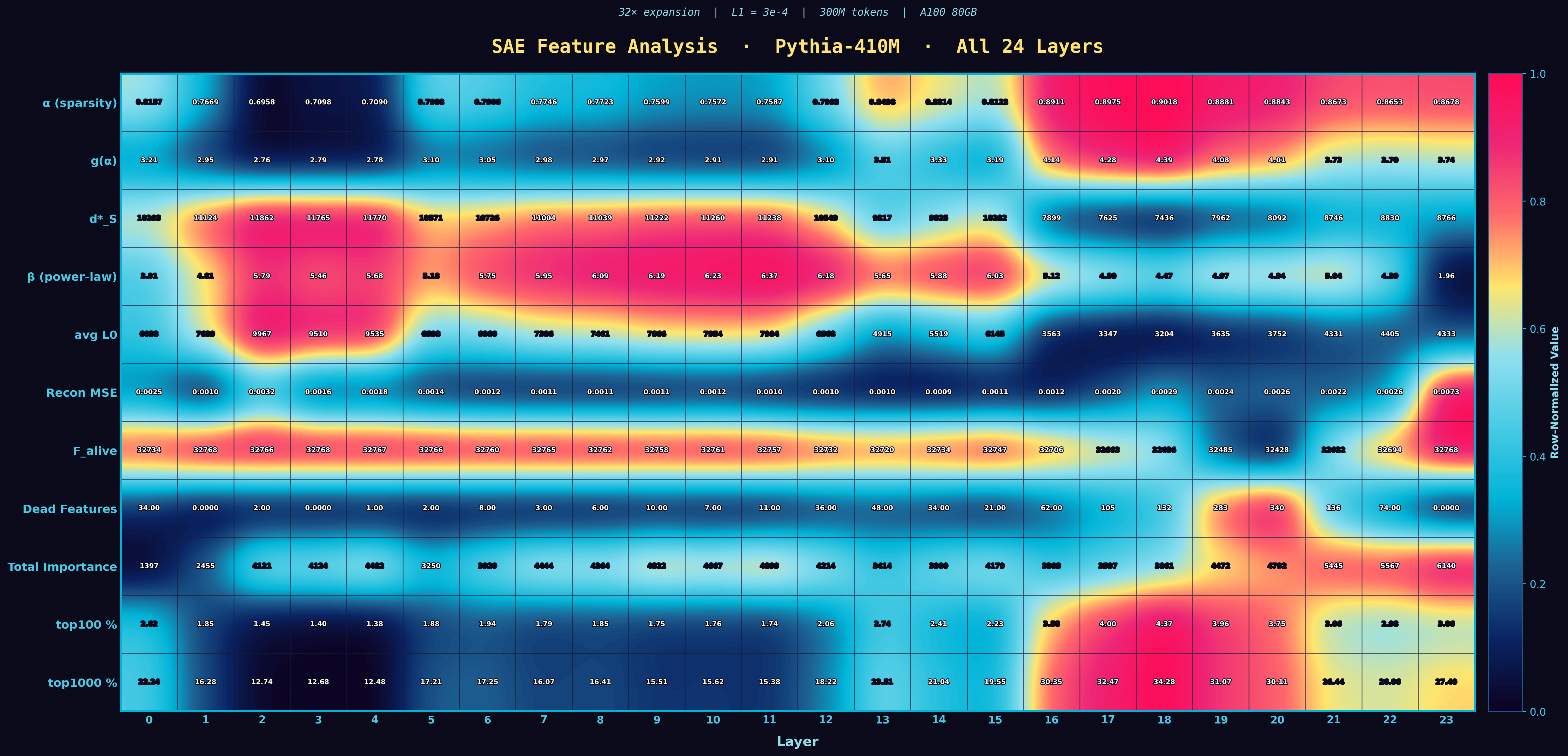
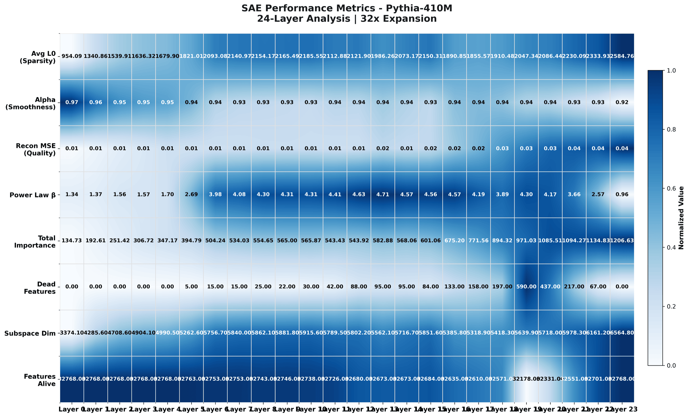
A compact summary card with one row per layer and one column per metric (L0, alpha, g(alpha), MSE, and so on). Shade tells you the relative value within the column. This is the at-a-glance shape of the whole trial.
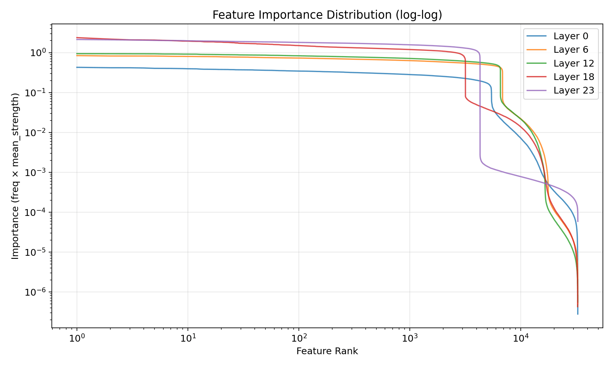
Feature-importance distribution from the earlier Erdős experiments. Tells you how attribution mass spreads across features rather than concentrating in a handful.
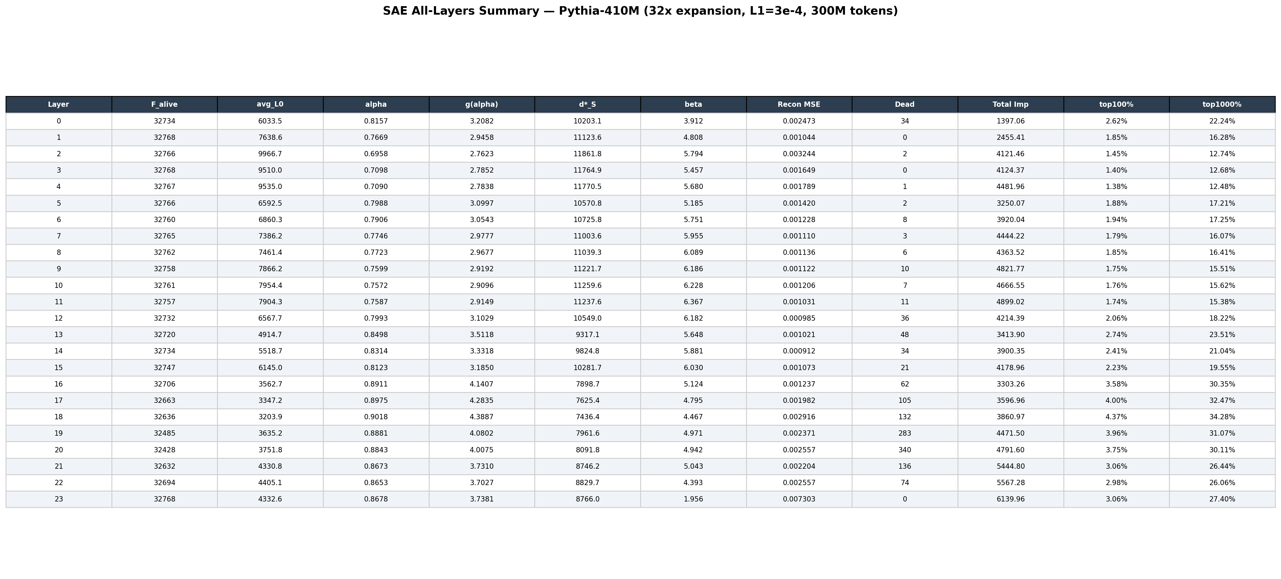
Per-layer summary table from the earlier experiments. The same kind of compact metric matrix that the SAE_Premium_Heatmap replaces in the newer work.
Earlier representation-learning experiment: the layer-by-feature heatmap rendered in a high-contrast cyberpunk style. Same shape of analysis as the later SAE heatmaps, just predating the KD framework that organises the new work.
Causal Dimensionality of Transformer Representations: Measurement, Scaling, and Layer Structure
Nilesh Sarkar, Dawar Jyoti Deka | arXiv Preprint
A study of how many causally effective dimensions a transformer's residual stream actually uses - measured via intervention rather than variance. The work tracks how this causal dimensionality scales with model size and how it is distributed layer by layer, connecting representation geometry to mechanistic interpretability.
Erdős AI Lab research spans knowledge distillation, interpretability, agentic AI, and world models, with work that has reached venues such as ICLR, NeurIPS, and ICCV.
SAE Experiments (KD paper)
Sparse Autoencoders (SAEs) are the central interpretability tool for the current knowledge-distillation paper. The work has two halves: a toy-model validation of the KD minimum-width theorem, then a real-LM sweep training 24 SAEs (one per Pythia-410M layer) for 300 M tokens at three different sparsity regimes. The full gallery below shows every figure produced for each trial, with notes on which variants made it into the paper and which did not. Also mirrored on the Interpretability Experiments page.
Experiment 1 - Toy-Model Validation
Before any real LM, a controlled toy environment validates the KD minimum-width theorem: theory predicts the dictionary width d*S at which reconstruction loss bottoms out. All three figures here go into the paper.
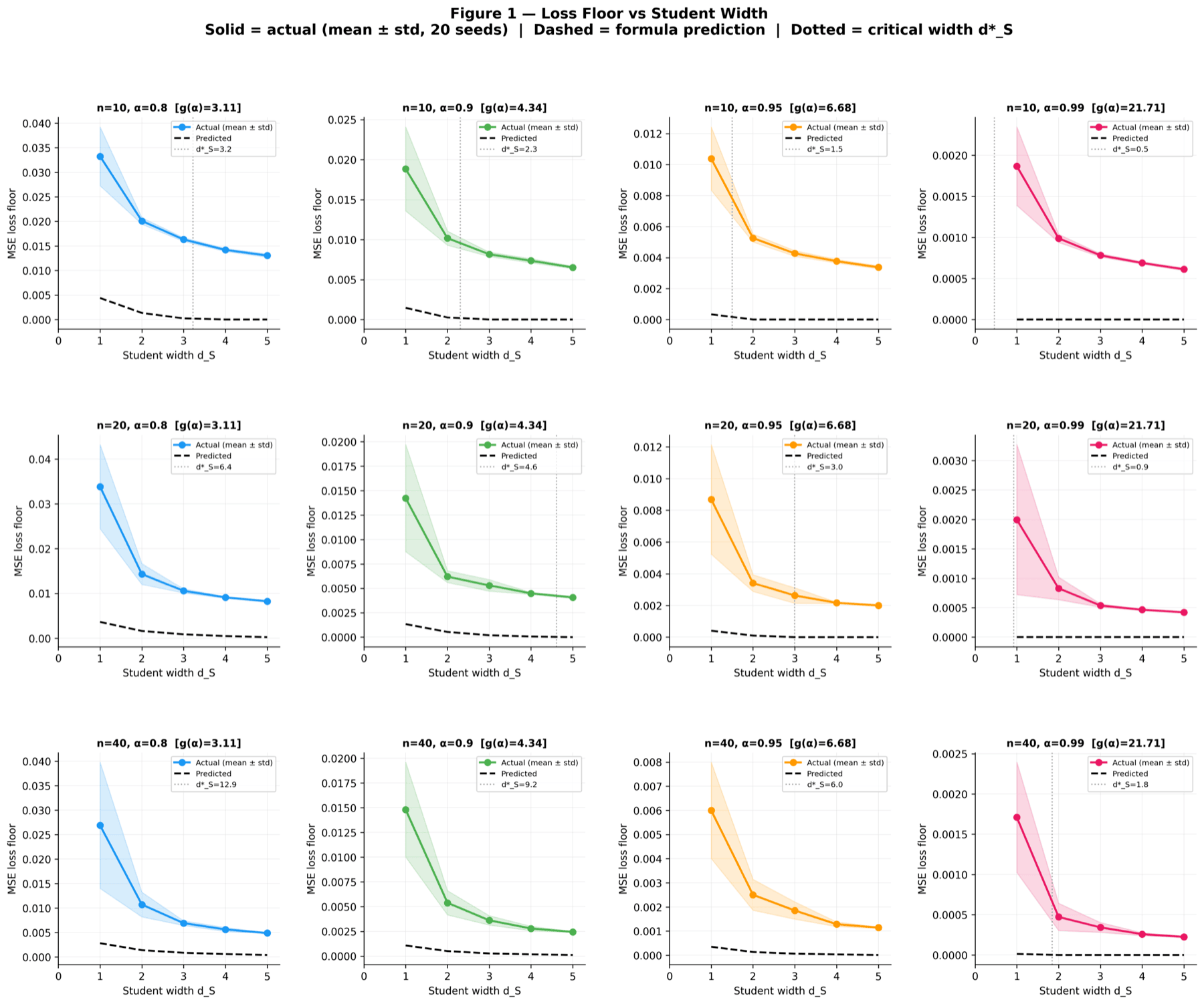
Each curve traces the reconstruction loss as the SAE dictionary width d_S grows, for a different (alpha, F) configuration. Theory predicts that loss hits a floor at the exact d*_S value, and the data agrees on every curve. This is the headline plot of the toy experiment because it shows the predicted minimum width is not just a tendency but a sharp transition.
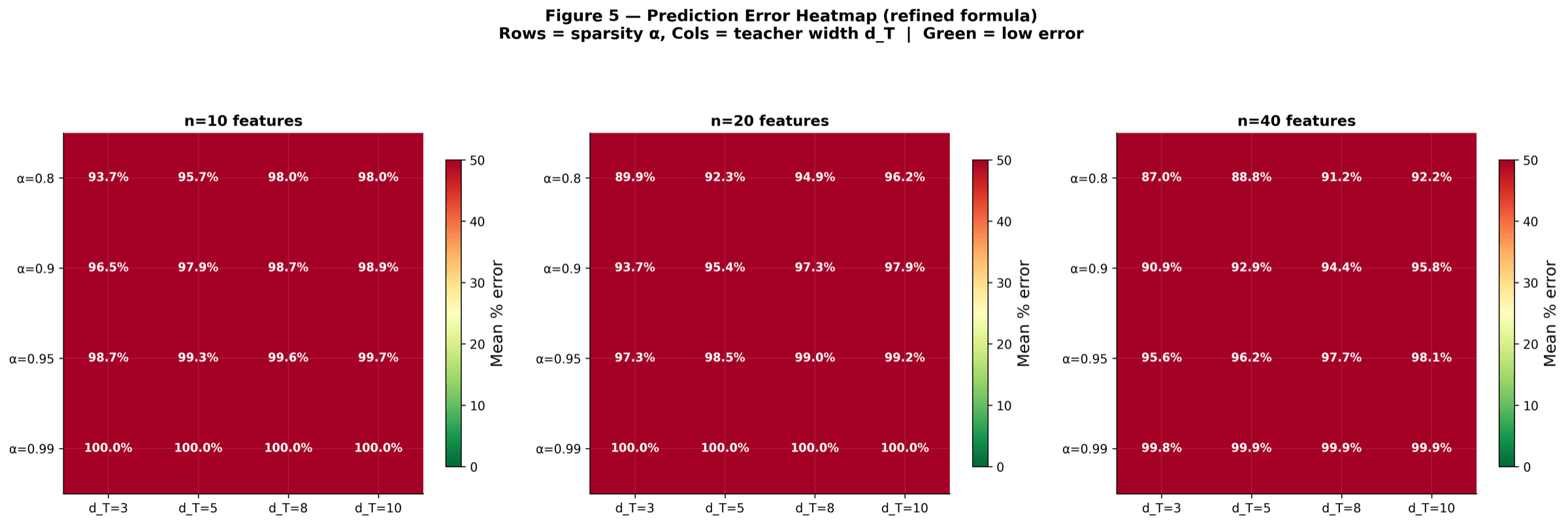
All (alpha, F) configurations on one canvas. Rows and columns sweep the two parameters; cell colour tells you how closely measured loss matches what KD theory predicted. Bright cells mean a near-perfect match. The point is to show the prediction holds uniformly across the parameter grid, not just on a handful of nice curves.
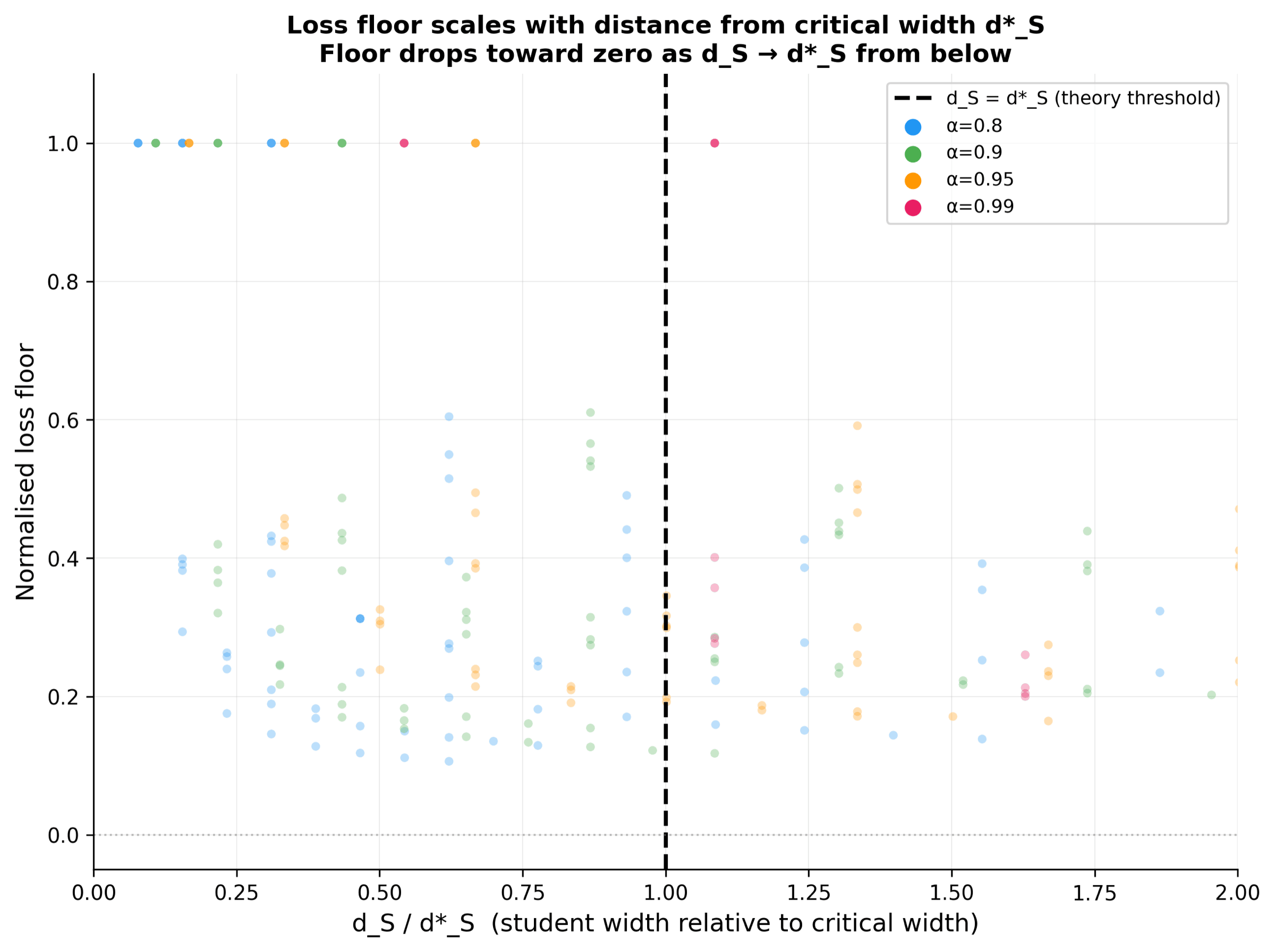
Every point compares the measured loss floor of a run to its theoretical d*_S value. If theory and experiment agree, the points sit on the y = x diagonal. They do. This single plot collapses the entire toy experiment into one image that says the theorem holds.
Trial A - L1 = 3e-4 fixed (dense regime)
Loosest sparsity. avg L0 ≈ 6,184, α ≈ 0.81, MSE ≈ 0.0019, d*S ≈ 9,963. Useful as a high-reconstruction baseline, not the regime for monosemanticity claims.

Reconstruction MSE, the L1 sparsity penalty, and the combined loss across all 24 SAE layers over 300 M training tokens. With L1 held loose at 3e-4 you get the densest activations (avg L0 around 6,184) and the best reconstruction. Each line is a layer, so the smooth simultaneous declines confirm no layer blew up.

A compact summary card with one row per layer and one column per metric (L0, alpha, g(alpha), MSE, and so on). Shade tells you the relative value within the column. This is the at-a-glance shape of the whole trial.
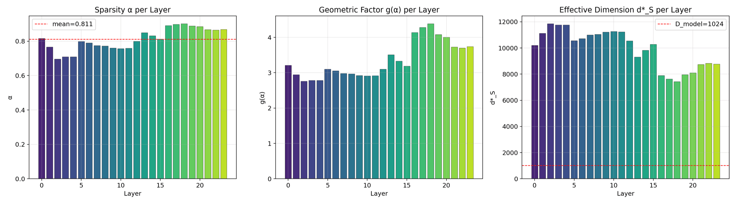
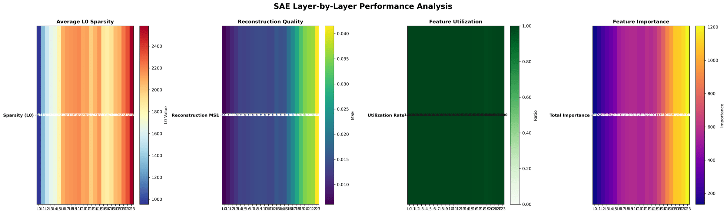
The three KD quantities plotted side by side per layer. Alpha measures sparsity, g(alpha) is the capacity function, d*_S is the predicted optimum dictionary width. These are the inputs theory needs to produce a width prediction.
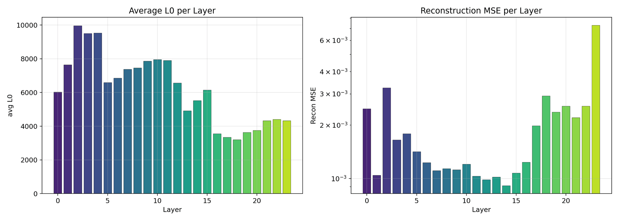
L0 (average active features per token) on one axis, reconstruction MSE on the other. Layers that are naturally denser sit on one side, sparser layers on the other. Reveals which transformer depths need more dictionary capacity.
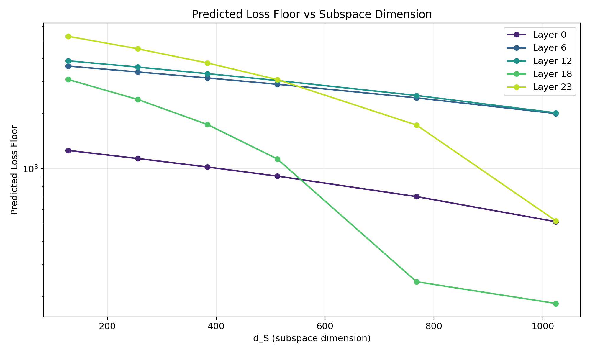
For each layer we sweep the dictionary width d_S and ask theory: where does loss bottom out? This figure draws the predicted curve. Comparing it against the actual training loss is what tells you the prediction is right.
Trial B - L1 = 8e-5 fixed (paper-exact)
Tuned so the L1 penalty matches the paper-exact sum formula. Seven rendering variants of the same per-layer measurements - chosen / rejected based on where each surface excels.
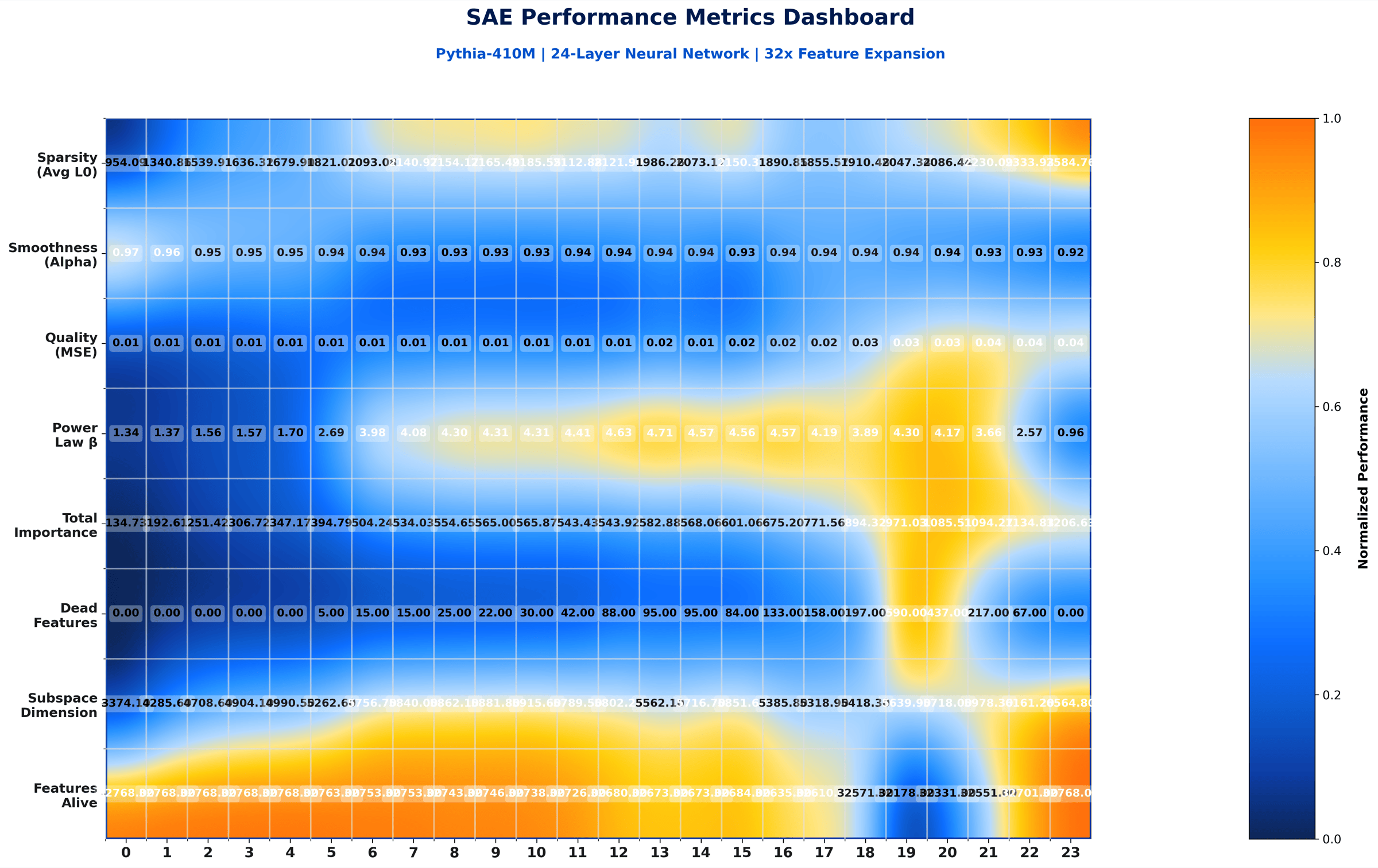
The clean paper-grade rendering of the L1 = 8e-5 paper-exact trial. Rows are layers, columns are SAE metrics. Annotated labels and a balanced palette are why this version was picked as the paper figure.
Same data as the premium heatmap, with a more compact and conservative palette. Built for LinkedIn cards and slide decks. Did not make the paper because the colour band is less expressive at print resolution.
Same data again, but each layer gets a sidecar with its own mini statistics. Used in the paper appendix where horizontal space is not as tight as the main column.
Small-multiples view: every layer's full metric vector tiled onto one page. Useful in show-me-everything talks where the audience wants to inspect each layer in isolation.
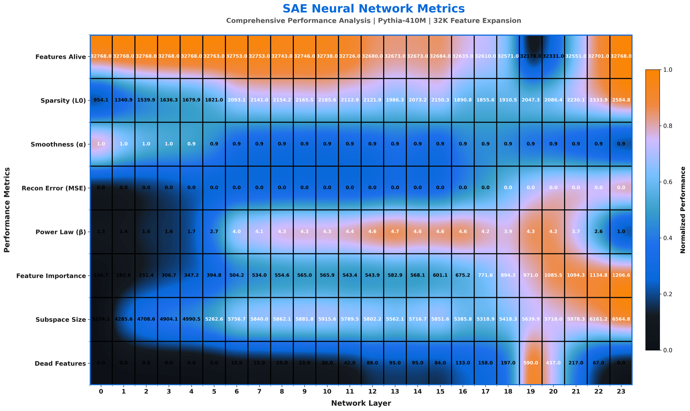
Smooth-gradient rendering of the same metrics. Looks great as a blog header, but the gradient hides exact bucket boundaries so it is harder to read off a precise number.
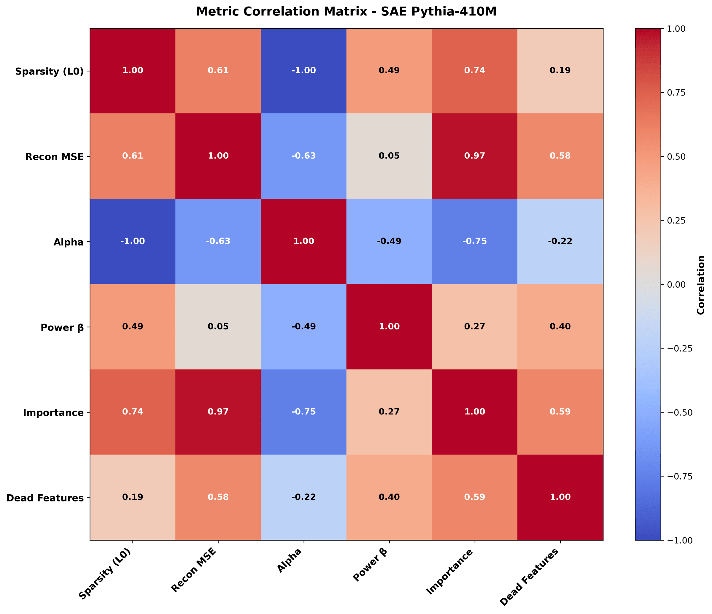
Which SAE metrics move together across layers. For example, alpha tracks dead-feature count. Useful for theoretical commentary about what each metric is really measuring.
Single card with the headline numbers: mean alpha, mean L0, total dead features. Used as the social and cover image, not as a paper-body figure.
Trial C - L1 = 5e-4 adaptive (target L0 ≈ 150)
Adaptive controller converges on L0 ≈ 152, α ≈ 0.994 - very sparse. ~7k dead features per layer but the survivors are doing real monosemantic work. Picked for the paper comparison panel precisely because the controller gives a guaranteed L0 target across trials.
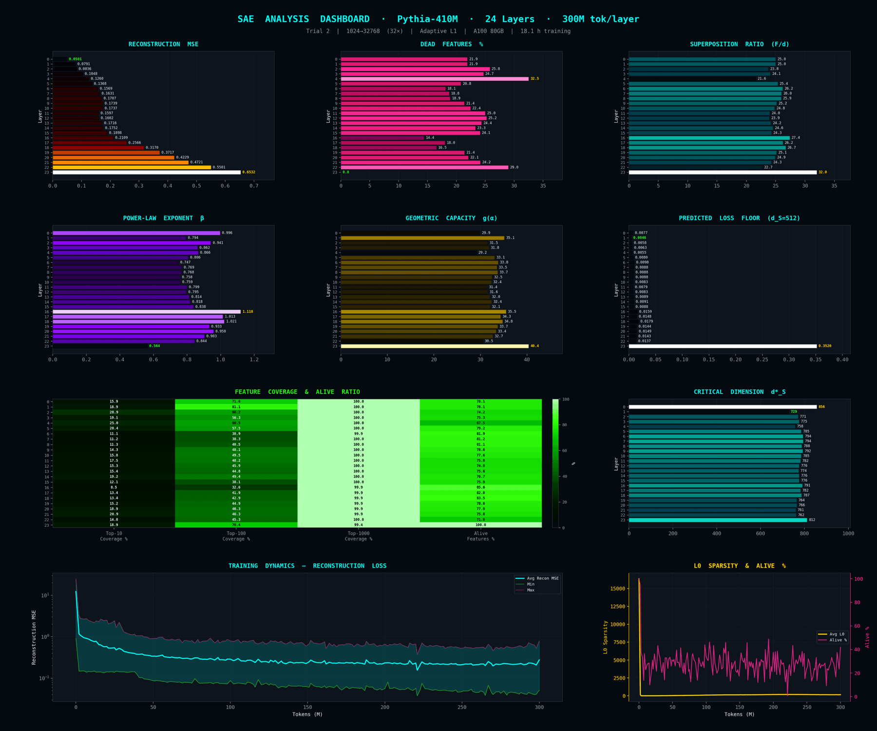
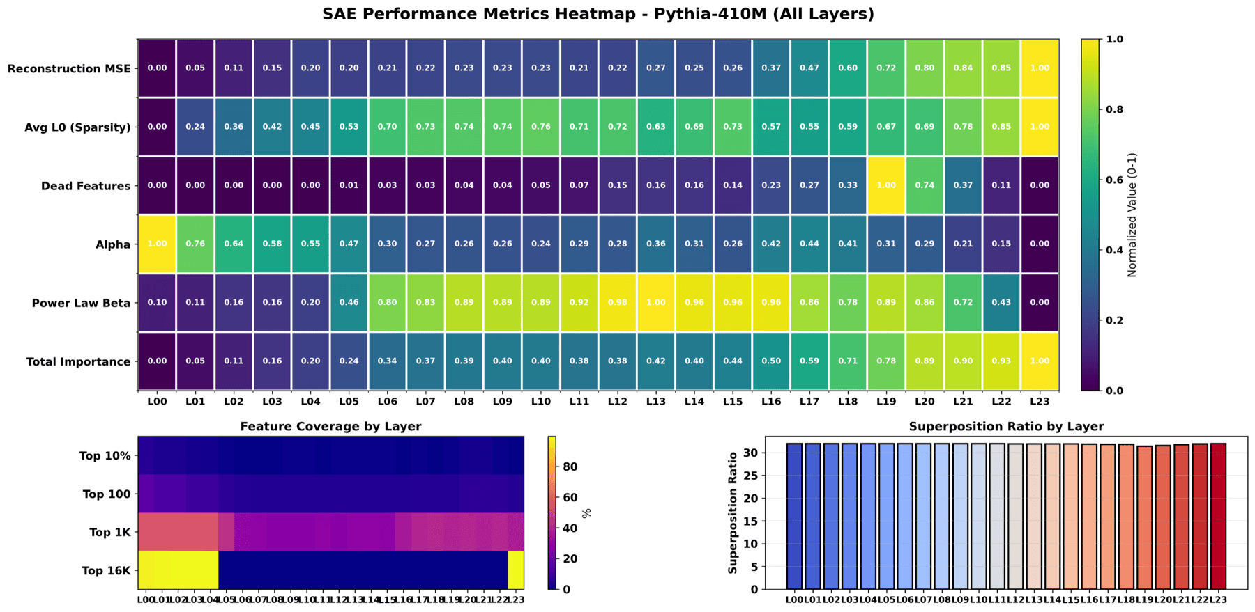
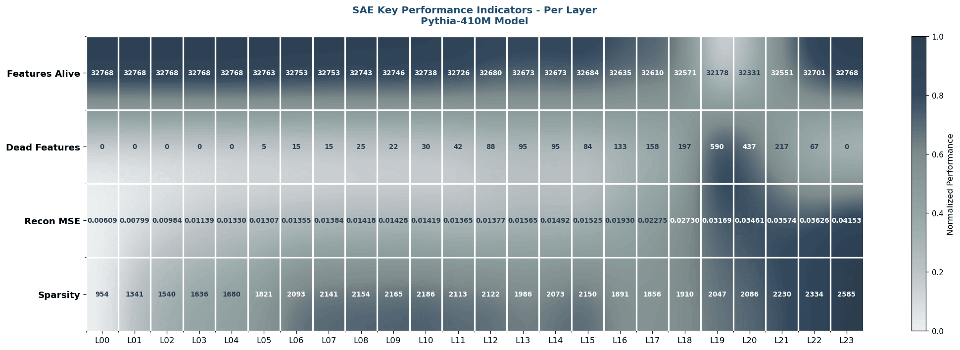
Dashboard view of the L1 = 5e-4 adaptive trial. Composite of alpha, g(alpha), reconstruction loss, dead-feature count arranged as a layer-by-metric grid. This is the figure the paper uses for the comparison panel because it carries hard numbers.
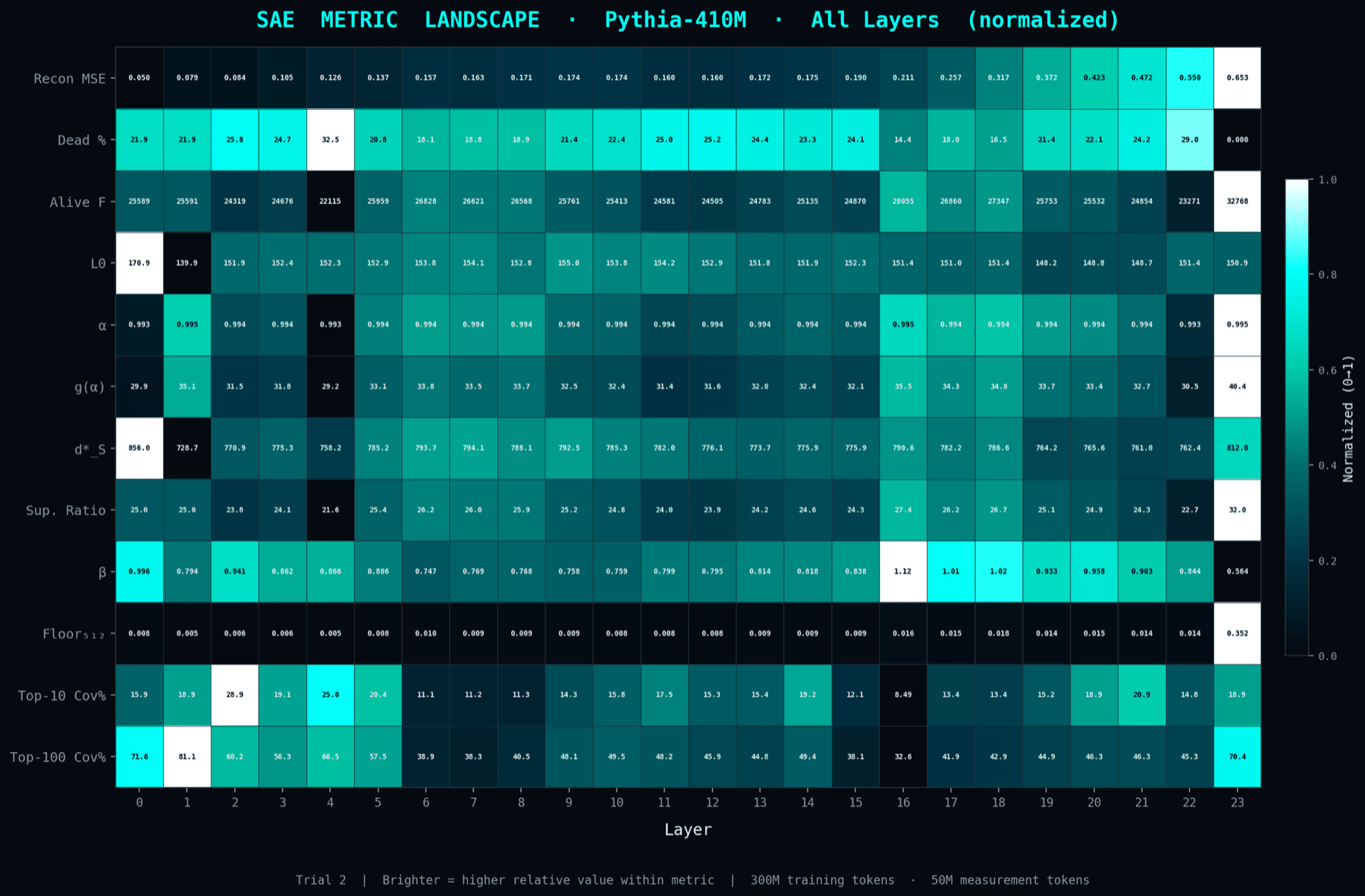
The same per-layer measurements rendered as a continuous landscape so you can read how each property evolves through depth. Qualitative but very quick to scan.
Why these three trials. Together they cover the corners of the sparsity-vs-reconstruction frontier the KD theory predicts: dense (3e-4), paper-exact (8e-5), very-sparse adaptive (5e-4 → L0 = 150). Other L1 settings (1e-4, 2e-4, 7e-4) were piloted but discarded - either redundant with an included trial or far outside the regime where KD applies.
Reproducibility. 144 checkpoints per trial (24 layers × 6 snapshots) on Hugging Face: colm-run-exp-2-t1 · colm-run-exp-2-t2 · colm-run-trial-2 · source on GitHub.