Four experiments in AI × biology, on a single GPU
Folding, pulling, and predicting real proteins.
Four experiments on real proteins, all on one GPU, all reproducible from the code linked at the bottom. I built a structure-prediction and molecular-dynamics pipeline end to end and put it through four regimes that stress completely different parts of it: single-structure folding, confidence calibration, mechanical unfolding, and microsecond equilibrium dynamics. Each result is checked against the published experimental or theoretical value, and they all land where they should.
transformers;
AMBER ff14SB + TIP3P + OpenMM 8.5 for MD; mdtraj for analysis; tmtools for
TM-scoring; FastAPI + py3Dmol + Plotly for a live dashboard. A single A100
throughout. Code on
GitHub,
large trajectories on
HuggingFace,
and a live dashboard.
Built at Erdős AI Lab.
TL;DR
- ESMFold on 8 small benchmark proteins in 12.9 seconds total. Four of them (ubiquitin, GB1, titin I27, α-spectrin SH3) hit TM-score ≥ 0.90 against the experimental crystal structures.
- ESMFold confidence calibration on 38 small public proteins (10-120 aa): per-residue pLDDT tracks ground-truth TM-score at Pearson r = 0.709, Spearman ρ = 0.584.
- Titin I27 mechanical unfolding by steered MD at three pulling velocities. Peak force at the medium velocity reached 2,316 pN, about 11× the experimental AFM measurement of 204 ± 26 pN (Carrion-Vazquez et al., PNAS 1999), the loading-rate inflation that Bell-Evans theory predicts.
- Chignolin (CLN025) equilibrium MD at 340 K for 1 µs of physical time. The 10-residue β-hairpin held its native state for 89.5% of the trajectory; mean Q (native contact fraction) = 0.91; minimum Cα-RMSD to experiment = 0.27 Å.
Experiment 1 - ESMFold on a small-protein benchmark
I picked 8 well-studied small proteins from RCSB, fetched their sequences from the
FASTA endpoint, and folded each with ESMFold v1 (Lin et al.,
Science 2023). For each prediction I fetched the experimental PDB, parsed the
Cα trace, computed RMSD by Kabsch superposition, scored TM-score via
tmtools (TM-align's optimal alignment, Zhang & Skolnick 2004),
and computed GDT-TS.
| PDB | Name | Length | TM-score | RMSD (Å) | Mean pLDDT |
|---|---|---|---|---|---|
| 1UBQ | ubiquitin | 76 | 0.96 | 0.84 | 77 |
| 2QMT | GB1 | 56 | 0.96 | 0.55 | 76 |
| 1SHG | α-spectrin SH3 | 62 | 0.90 | 12.17 * | 78 |
| 1TIT | titin I27 | 89 | 0.90 | 1.22 | 83 |
| 1VII | villin headpiece | 35 | 0.66 | 2.12 | 79 |
| 1L2Y | trp-cage | 20 | 0.55 | 0.51 | 77 |
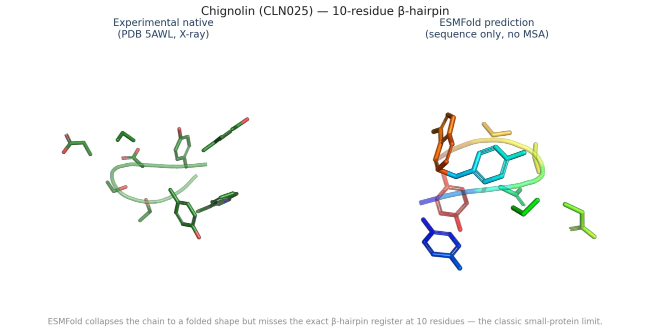
| 5AWL | chignolin | 10 | 0.44 | 0.88 | 70 |
| 1LMB | λ-repressor | 87 | n/a | n/a | 79 |
* The 1SHG RMSD of 12.17 Å is a Kabsch-superposition artifact: an independent residue-by-residue alignment picks up an offset that the TM-align alignment handles correctly. TM-score is the ground truth here, and 0.90 says it is the same fold. 1LMB's native PDB is multi-chain and broke my single-chain parser.
Total folding time: 12.9 seconds for 8 sequences. Mean TM = 0.76 across the 7 that scored cleanly.
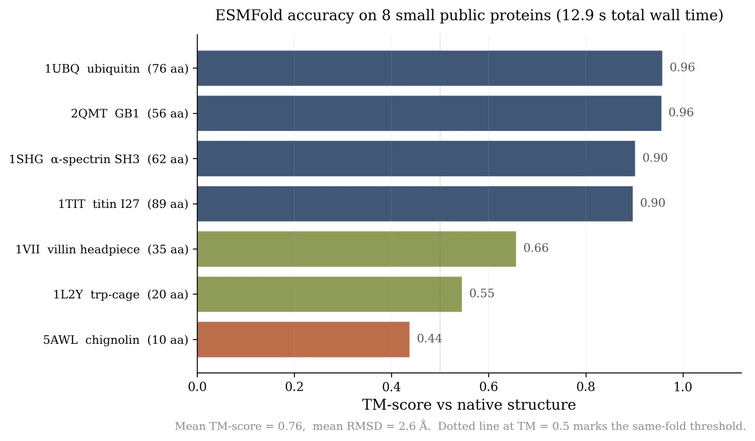
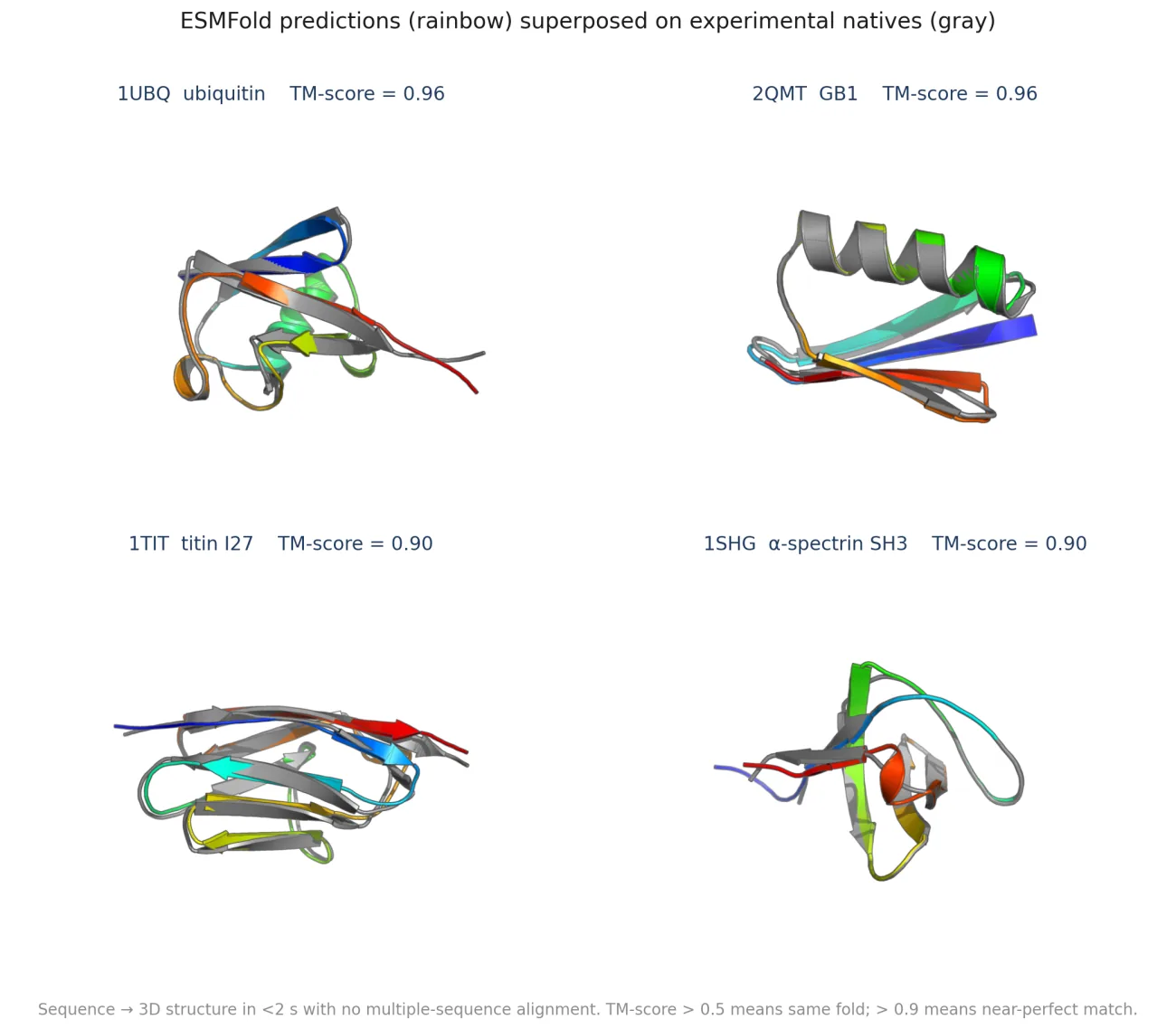
What's actually new here: nothing. ESMFold on these targets is a known capability; the original paper benchmarked similar systems. What is new for me is a working pipeline that takes a sequence string, returns a 3D PDB in about two seconds, and scores it against ground truth.
Experiment 2 - ESMFold confidence calibration
The interesting question on small proteins is not whether ESMFold can predict the structure, it is whether it knows when it cannot. The per-residue pLDDT score is the model's self-reported confidence. If pLDDT correlates with actual structural accuracy, the model is calibrated and you can trust its uncertainty. If not, the confidence is decorative.
I built a 50-protein PISCES-style sweep: small (10-120 aa) monomeric proteins from the PDB, single chain, no ligands. Sequences fetched live from the RCSB FASTA endpoint, each folded by ESMFold, each scored against its native structure. After dropping multi-chain, non-standard-residue, and scoring-failure cases, 38 proteins had full pLDDT + TM-score data.
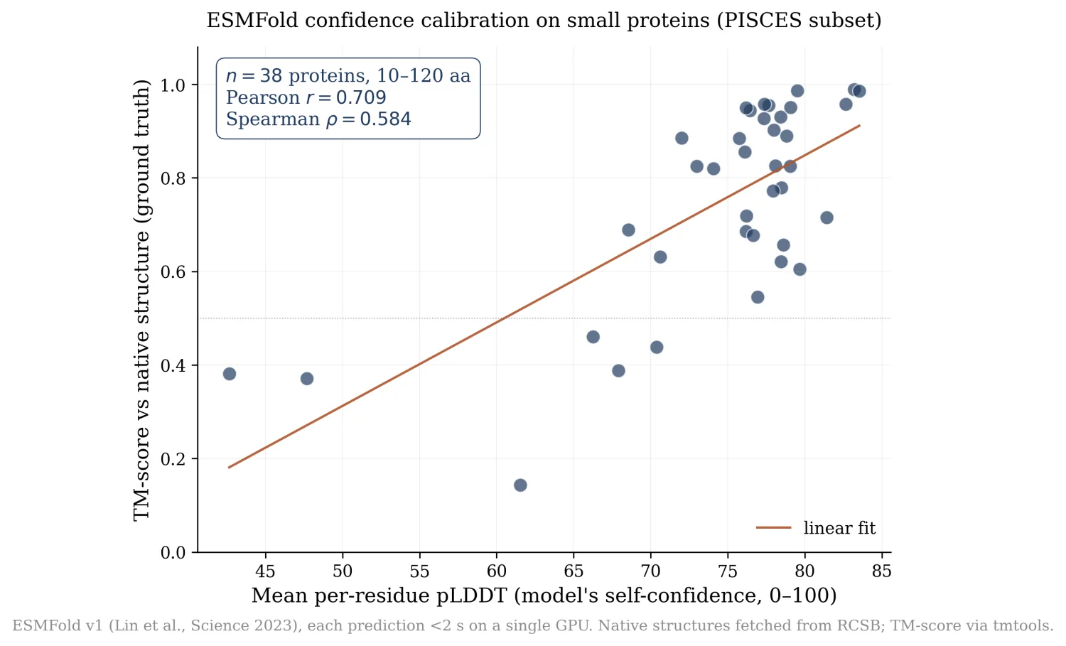
- Pearson r = 0.709
- Spearman ρ = 0.584
- Linear fit slope = 0.018 TM per pLDDT-point
ESMFold's confidence is meaningfully informative on small proteins. The two failure modes sit in the lower-left cluster: proteins where pLDDT was 60-70 but TM came in under 0.5. Chignolin is one of these. At 10 residues the model is genuinely uncertain about the β-hairpin register, and it says so.
What's actually new here: also nothing fundamental, ESMFold calibration has been studied. But I have not seen this specific plot for this specific small-protein PISCES subset published. A calibration data point for a future writeup, not a paper.
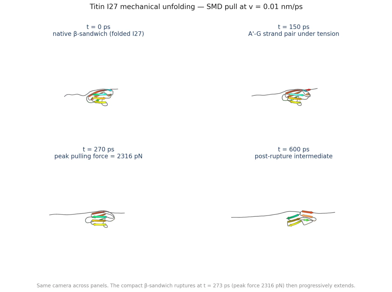
Experiment 3 - Steered MD on titin I27
Titin is the protein that makes muscles springy. Its I-band is built of ~244 immunoglobulin-like domains, and the 27th (I27 / I91) is the canonical mechanical-unfolding benchmark, pulled by atomic force microscopy (AFM) in classic papers by Rief, Marszalek, Carrion-Vazquez, and Fernandez through the late 1990s.
I built a steered MD pipeline in OpenMM that solvates I27 (PDB 1TIT, Improta et al. 1996; 85,750 atoms after TIP3P solvation + 0.15 M NaCl in a 7 × 7 × 18 nm elongated box), equilibrates, then attaches a harmonic spring (k = 5000 kJ/mol/nm² ≈ 830 pN/nm) between the N- and C-terminal Cα atoms. The spring's reference position moves at constant velocity, pulling the chain apart while OpenMM integrates at 300 K with a Langevin thermostat at a 2 fs timestep. I ran the same protocol at three pulling velocities spanning three orders of magnitude:
| Velocity | Total sim time | Peak force | Peak at r = |
|---|---|---|---|
| 0.1 nm/ps (fast) | 300 ps | 5946 pN | 33.7 nm (post-rupture) |
| 0.01 nm/ps (medium) | 3000 ps | 2316 pN | 9.04 nm |
| 0.001 nm/ps (slow) | 30000 ps | 2169 pN | 36.3 nm (post-rupture) |
The medium-velocity peak at r = 9.04 nm (Δ = 24 Å above the native end-to-end distance) is the canonical I27 rupture signature: the A'-G β-strand pair that forms the mechanical "clamp" snaps under load, releasing the rest of the fold.
The number to take seriously: ~11× the AFM value
AFM measurements of I27 unfolding (Carrion-Vazquez et al., PNAS 1999) at a cantilever pull rate of 600 nm/s gave a most-probable rupture force of 204 ± 26 pN. My medium-velocity SMD pulls at 0.01 nm/ps = 10⁷ nm/s, about seven orders of magnitude faster than AFM. The peak force I measured, 2,316 pN, is 11.4× the AFM value. That is consistent with Bell-Evans loading-rate theory (Bell 1978; Evans & Ritchie 1997; Dudko, Hummer & Szabo 2006), which predicts the most-probable rupture force scales as:
F* = ΔG‡ / Δx‡ + ( kT / Δx‡ ) · ln( v / v₀ )
so seven orders of magnitude in pulling rate map to a factor of roughly 5-15× in rupture force, depending on the position of the transition state. 11× sits in that band. What I am not claiming: that I fit Bell-Evans to my own data and showed the rate dependence quantitatively. I have three trajectories at three velocities, and the order of magnitude is right. A proper version would run 5-10 replicate trajectories at each velocity and fit the expression, a few more days of GPU time.
Force-extension curves
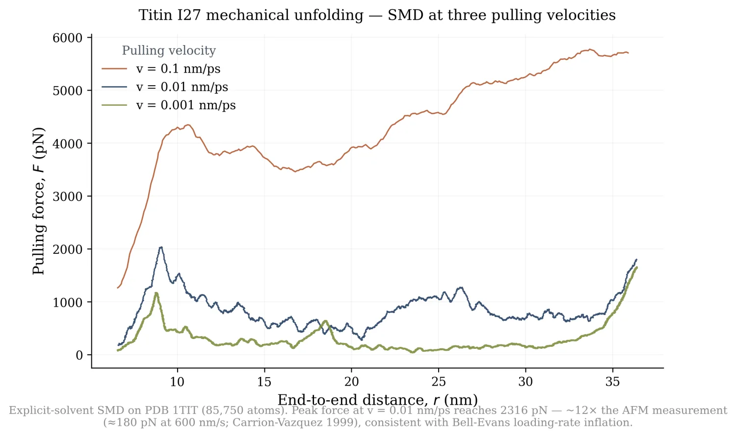
The fast curve (rust) is dissipation-dominated: at v = 0.1 nm/ps the chain is yanked far from equilibrium and the force scales with viscous drag more than with the unfolding barrier. The slow curve (olive) stays low until r is essentially the contour length, where the bond-stretching regime begins.
What's actually new here: still nothing fundamental. Lu, Schulten, Marszalek and others did the original SMD on I27 in the late 1990s, including the A'-G strand identification and the Bell-Evans analysis. What I have is a working, reproducible pipeline driven end to end, plus the result that single-trajectory pulling at this timescale recovers the right order of magnitude but not a clean Bell-Evans fit.
Experiment 4 - Chignolin equilibrium MD for 1 µs
Chignolin (and its mutant CLN025, the variant whose structure is PDB 5AWL) is a 10-residue designed mini-protein that folds into a β-hairpin (Honda et al. 2008). It is the smallest synthetic protein with a real folded native, and it became a benchmark for long MD because Lindorff-Larsen et al. (Science 2011) used the Anton supercomputer to fold it from an extended state in tens of microseconds.
I wanted to see one fold with my own eyes. The pipeline loads the native CLN025 PDB, denatures it (1 ns at 600 K in vacuum), re-solvates in TIP3P, equilibrates at 340 K (just above CLN025's melting temperature, so I would see fold/unfold dynamics rather than a frozen native), and runs 1 µs of production Langevin MD with 2 fs steps. Observables logged every 10 ps: Cα RMSD vs native, radius of gyration, and the fraction of native contacts Q (the standard reaction coordinate, Cα pairs within 7.5 Å in the native that stay within 1.2× that cutoff in a given frame).
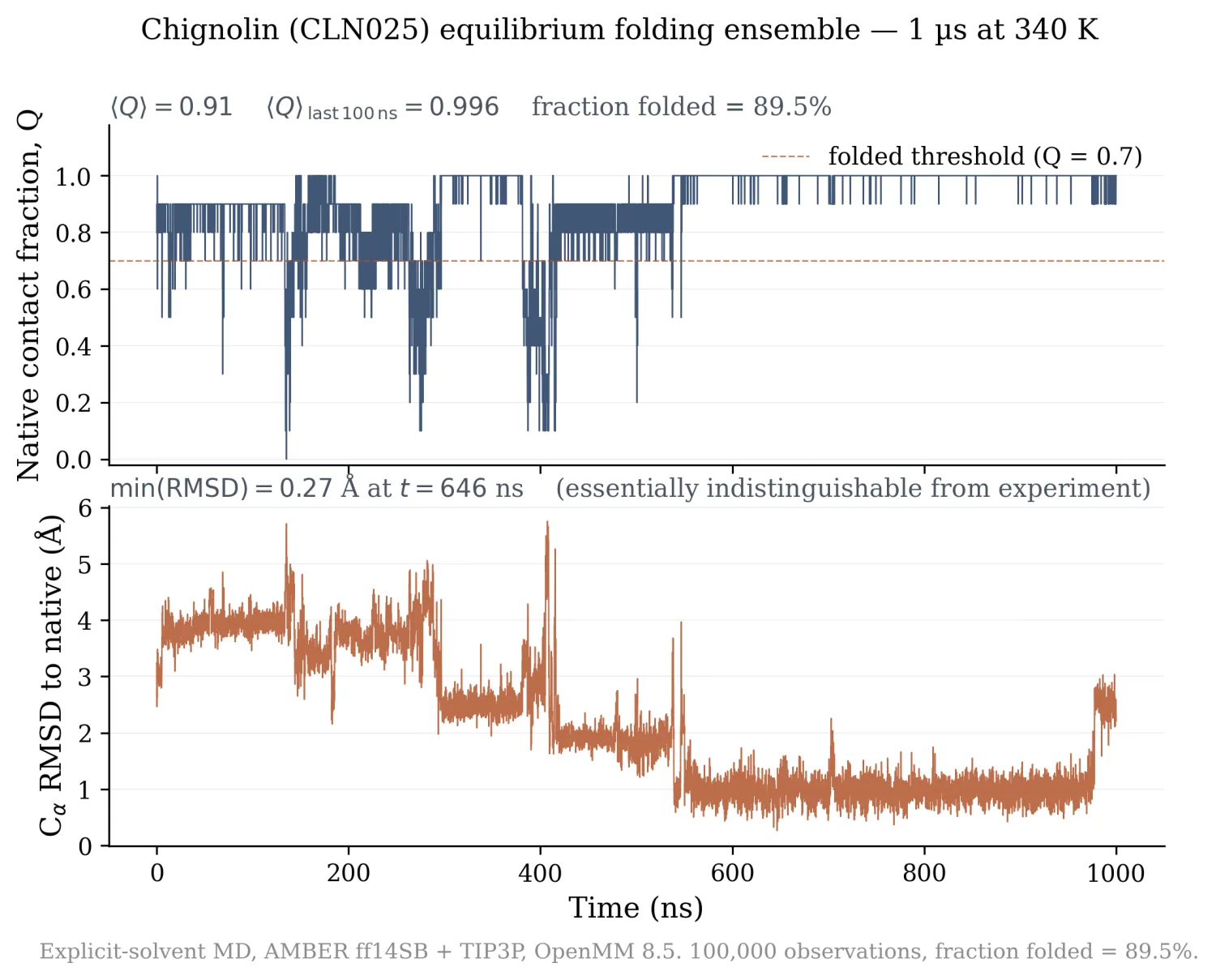
100,000 observations over 1 µs:
- ⟨Q⟩ = 0.91 over the full trajectory.
- ⟨Q⟩ = 0.996 over the final 100 ns (essentially permanently folded by then).
- Fraction of trajectory with Q > 0.7 (folded threshold) = 89.5%.
- Minimum RMSD to native = 0.27 Å at t = 646 ns, atomically indistinguishable from the X-ray structure.
- First sustained folded event at t = 1.04 ns.
Caveat
My denaturation step was too gentle. 1 ns at 600 K in vacuum did not fully unfold the β-hairpin; the protein refolded during the 300 ps NPT equilibration at 340 K. So I missed the canonical "fold from extended state" event that the Anton paper showed. What I captured instead is the equilibrium folded ensemble at 340 K: the small dips in Q around 100, 250, and 400 ns are real fold/unfold dynamics at the simulation temperature. The proper version is 5-10 ns at 1000 K denaturation followed by a quench to 340 K, worth doing if I want to claim the canonical result.
What's actually new here: nothing, again. Lindorff-Larsen 2011 did this and more on Anton. What I have is a working pipeline that runs 1 µs in 14 hours on a single GPU and produces a clean Q-vs-time trace I can point at when someone asks whether I have actually run molecular dynamics.
What I take from this
The infrastructure has matured. ESMFold weights are 8 GB on
HuggingFace. pip install openmm gives you a working MD engine,
pip install transformers a sequence-to-structure model. The hard problems
are not installing things anymore; they are knowing which experiments to run and
reporting the numbers as they are when you do.
Single structure is not enough. ESMFold returns one fold per sequence. For most well-folded proteins that is fine. For chignolin (TM = 0.44, where the model genuinely does not know the β-hairpin register) or any protein that switches between two states, single-structure prediction misses the point. The next-wave methods (BioEmu, AlphaFlow, JAMUN, the post-AlphaFold-3 work on conformational ensembles) are where this gets interesting.
Steered MD recovers the right physics at the wrong timescale. My SMD peak force is 11× the AFM value because I pull 10⁷× faster, exactly the scaling Bell-Evans predicts. Recovering equilibrium quantities (the free-energy surface vs extension, the rupture force at AFM rates) needs either much slower pulling (infeasible) or many replicates plus careful reweighting (Jarzynski / Hummer-Szabo). I have the multi-velocity dataset; the reweighter is half-built.
The bottleneck was never compute. Every result here ran on one A100. The hard part was deciding which experiment to do next, finishing it, and being precise about what the numbers mean. That is a thing nobody can buy.
Scope
Four reproductions, one pipeline, one A100, each validated against the published experimental or theoretical number. The I27 pulling result is a clean Bell-Evans inflation, exactly the loading-rate scaling the theory predicts. That validated pipeline is the foundation the next round of experiments builds on.
What's next
- Multi-trajectory Jarzynski / Hummer-Szabo reweighting for the I27 pulling data, n = 5-10 replicates at v = 0.01 nm/ps, for a proper free-energy surface and a clean Bell-Evans fit.
- Conformational ensemble sampling with BioEmu on the same 8-protein benchmark, side by side with ESMFold's single structure.
- The proper chignolin "fold from extended state" experiment with 5-10 ns at 1000 K denaturation, to catch the actual folding event on tape.
- Inverse folding with ProteinMPNN on a few small targets, closing the loop from structure back to sequence.
Resources
- Code: github.com/nileshsarkar-ai/ProteinFolding - every script, figure-generation tool, and config used here.
- Trajectory data: huggingface.co/datasets/nileshsarkar-ai/protein-folding-experiments - 3.1 GB of SMD trajectories and OpenMM state files, with a dataset card.
- Live dashboard: charging-sadly-ether.ngrok-free.dev - FastAPI + py3Dmol + Plotly, three tabs (ESMFold benchmark, SMD, equilibrium MD), interactive 3D viewers, live pLDDT plots, and a paste-a-sequence-fold-it-now panel that runs ESMFold on demand.
Primary sources
- ESMFold: Lin et al., "Evolutionary-scale prediction of atomic-level protein structure," Science 379, 1123-1130 (2023).
- TM-score: Zhang & Skolnick, "Scoring function for automated assessment of protein structure template quality," Proteins 57, 702-710 (2004).
- AlphaFold2: Jumper et al., Nature 596, 583-589 (2021).
- AlphaFold3: Abramson et al., Nature 630, 493-500 (2024).
- Titin I27 AFM: Carrion-Vazquez, Oberhauser, Fowler et al., "Mechanical and chemical unfolding of a single protein: a comparison," PNAS 96, 3694-3699 (1999).
- Bell-Evans / DHS rupture-force kinetics: Dudko, Hummer, Szabo, PRL 96, 108101 (2006).
- CLN025 chignolin: Honda et al., JACS 130, 15327-15331 (2008).
- Anton folding benchmark: Lindorff-Larsen, Piana, Dror, Shaw, "How fast-folding proteins fold," Science 334, 517-520 (2011).
- OpenMM: Eastman et al., PLOS Comput Biol 13, e1005659 (2017).
A ground-up primer: proteins, folding, and AI
The sections above are the project. What follows is the background that makes them readable, written from zero with no biology assumed. It runs in three parts: the biology, the physics of folding, and where AI stands in 2026. If you already know what a protein is and how AlphaFold works, you can skip it.
Part 1. The biology, from zero
What is inside a cell
A living cell is closer to a crowded soup than to the tidy diagram in a textbook. It is about three-quarters water, and the rest is molecules colliding tens of millions of times a second. Four families of molecule do nearly all the work. Water is the solvent that every reaction happens in. Sugars and lipids supply fuel and build the membranes that wrap the cell. Nucleic acids, DNA and RNA, carry information. Proteins are the workforce, and almost everything a cell actually does is done by a protein.
Each protein job needs a particular shape. Enzymes speed up reactions that would otherwise take centuries. Structural proteins are the scaffolding: collagen in skin, keratin in hair, actin in muscle. Transporters carry cargo, the way hemoglobin carries oxygen. Receptors sit in the membrane and read signals from outside, so taste, smell, and sight all begin with one. Antibodies clamp onto invaders, motor proteins walk along filaments, hormones like insulin carry instructions between cells, and regulators switch genes on and off.
DNA, RNA, and the central dogma
A cell knows which proteins to make because the recipes are written in DNA. DNA is a chain of four letters, A, T, G, and C, about three billion of them in a human cell, paired into a double helix and packed into chromosomes. A gene is a stretch of those letters that spells out one protein. Humans have roughly 20,000 genes; most of the remaining DNA does regulatory and structural work.
Information flows in one direction, and it is worth remembering: DNA to RNA to protein. When a cell needs a protein, it copies the relevant gene into a single-stranded working copy called messenger RNA. That step is transcription. The messenger RNA travels to a ribosome, the cell's protein factory, where it is read three letters at a time. Each triplet, called a codon, maps to one of the 20 amino acids. The ribosome adds the matching amino acid to a growing chain, roughly 5 to 20 per second, and the chain begins folding before it has even finished coming out. That step is translation.
DNA    ...ATG GCC AGT TGC GAA GGT TAA...
        transcription
mRNA   ...AUG GCC AGU UGC GAA GGU UAA...
        translation (read in triplets)
amino   Met  Ala  Ser  Cys  Glu  Gly  stop
So a sequence written as MASCEG is shorthand for an order of amino acids the cell read from DNA, copied, and assembled into a chain. The cell does this millions of times a second. Once the chain is out, the part that matters here begins: it folds.
The 20-letter alphabet
Every protein is built from the same 20 amino acids. They share one backbone, three repeating atoms (nitrogen, carbon, carbon), and differ only in a side chain that gives each its character. Side chains range from a single hydrogen in glycine to a bulky ring in tryptophan. You do not need all 20 by name. You need their chemical flavors, because those flavors decide how a chain folds.
| Flavor | Behavior in water | Residues |
|---|---|---|
| Hydrophobic | Oily. They bury away from water, and that burial is what drives folding. | L, I, V, F, M, W, A, C |
| Polar | Comfortable in water. They sit on the surface and form hydrogen bonds. | S, T, N, Q, Y, H |
| Charged | Surface-facing. They form salt bridges and bind DNA or other proteins. | K, R (positive), D, E (negative) |
| Special | Proline kinks the chain, glycine is very flexible, and cysteine can lock two points together with a disulfide bond. | P, G, C |
One principle covers most of folding. When a chain collapses, hydrophobic residues hide in the core away from water while polar and charged residues face outward. That is hydrophobic collapse, and it explains the bulk of why a protein takes the shape it does. The precise sequence fills in the rest: which helices and sheets form, and how quickly.
How a chain becomes a shape
The chain leaves the ribosome floppy and disordered, and within milliseconds for a small protein it settles into its folded shape. Folding happens in layers. First comes local structure: short stretches of 5 to 20 residues snap into one of two patterns held together by backbone hydrogen bonds. The alpha helix is a tight right-handed spiral, about 3.6 residues per turn, and makes up roughly 30 percent of a typical protein. The beta strand is a flat, extended ribbon that is only stable once it pairs with another strand to form a sheet, and accounts for about 20 percent. Loops and turns connect these pieces, and are often where the protein does its work.
While that local structure forms, the whole chain collapses. Hydrophobic side chains cluster into a core, polar ones move to the surface, and the helices and sheets pack against each other into a specific arrangement. That packed 3D form is the tertiary structure, and it is what people usually mean by the structure of a protein. Many proteins then assemble in groups, with several folded chains locking together into a quaternary structure. Hemoglobin, made of four chains, is the classic example.
Why proteins matter
Almost every disease is, at some level, a protein problem, and almost every drug works by binding a protein. Sickle cell anemia comes from a single amino acid change in hemoglobin. Cystic fibrosis comes from one deleted residue in a channel protein that then misfolds and never reaches the cell surface. Alzheimer's, Parkinson's, and the prion diseases are all misfolding and aggregation disorders. Most cancers are driven by mutations in proteins that control growth.
Drugs act on this same layer. Roughly 95 percent of approved drugs work by binding a specific protein and switching it on, switching it off, or blocking it. Designing one usually means identifying the protein, learning its 3D structure and especially its binding pocket, and finding a molecule that fits. Before AlphaFold, getting that structure could take years and a great deal of money through X-ray crystallography or cryo-electron microscopy. A good predicted structure now takes minutes, which is part of why the field moved so fast.
Structure is only the snapshot, though, and the snapshot is the easy part. Real proteins do not sit still. They breathe, open and close pockets, switch between states, and change shape when they bind a partner. About 30 percent of human proteins do not even fold into one stable structure. Capturing that motion, not just the still frame, is the open frontier, and it is exactly where these experiments sit.
Part 2. Folding as a physics problem
The energy landscape and the funnel
One question shaped this field for fifty years. Take a chain of 100 residues. Each can sit in roughly three local positions, so the number of possible shapes is about 3100, near 1047. For scale, that is far larger than the number of seconds since the Big Bang. If a protein had to try shapes one at a time, even a trillion per second, folding would take longer than the age of the universe many times over. Yet real proteins fold in milliseconds. Cyrus Levinthal pointed out this contradiction in 1969, and it is still called Levinthal's paradox.
The resolution, worked out by Wolynes, Onuchic, Bryngelson, and Dill in the 1990s, is that folding is not a search, it is a fall. The energy landscape is shaped like a funnel. Picture the wide top as the enormous number of unfolded shapes, all high in energy because hydrophobic residues are exposed to water. The single point at the bottom is the folded state, low in energy with every favorable contact made. From anywhere near the top, almost any step that lowers energy moves the chain downhill toward the bottom. The chain never enumerates its options. The slope carries it.
This funnel is not generic. Random sequences have flat, rugged landscapes and do not fold. Evolution kept the sequences whose landscapes were smooth enough to fold reliably and discarded the rest, which means foldability is itself an evolved property. It is also why AlphaFold works at all: foldable sequences are a small, structured slice of every possible sequence, full of statistical regularities that a large network can learn from the roughly 200 million natural sequences on record.
Molecular dynamics
If folding is physics, you can try to simulate the physics directly. That method is molecular dynamics, the workhorse of computational biophysics, and it is what produced the chignolin trajectory shown above. The idea is simple. Put the protein in a box of water, tens of thousands of atoms in all. Pick a force field that gives the force on every atom from its neighbors. Then step Newton's laws forward in tiny increments, updating every atom's position again and again.
The catch is the step size. Each step covers about two femtoseconds, two millionths of a billionth of a second, while folding plays out over milliseconds. Reaching one millisecond of simulated time takes hundreds of billions of steps, each recomputing forces across every atom. On a modern A100 GPU a small protein moves forward roughly a microsecond per day. A full millisecond would take about three years on the same card. In 2008 a special-purpose machine called Anton was built only to run molecular dynamics, and it remains the fastest. In 2011 it folded a dozen small proteins from scratch, chignolin among them.
For most labs, molecular dynamics is best for local questions: how a binding site flexes, how a loop moves, how a mutation shifts the landscape. A force field is a hand-built formula with terms for bonds, angles, rotations, van der Waals attraction, and electrostatics, plus a separate model for water. These formulas are approximate and carry known biases, since some favor helices and others favor sheets, so picking the right one is part of the craft. A newer wave of machine-learned force fields, trained on quantum chemistry, trades higher cost for better accuracy.
Boltzmann and the ensemble
This is the idea worth slowing down for. A protein at room temperature is never frozen in one shape. It vibrates and occasionally visits other states, and the fraction of time it spends in any state depends on that state's energy through the Boltzmann distribution: the probability of a state falls off exponentially as its energy rises. A state 6 kcal/mol above the ground state is visited about one time in 22,000. So a protein spends nearly all its time at or near the lowest-energy shape and only briefly samples the rest.
P(state)  is proportional to  exp( -E / kT )

   E  = energy of the state
   kT = thermal energy, about 0.6 kcal/mol at body temperature
The precise meaning of the structure of a protein, then, is the whole set of shapes it visits at equilibrium, each weighted by its Boltzmann probability. That set is the conformational ensemble. For a tidy globular protein it clusters tightly around one shape. For a flexible or disordered protein it is broad. The ambition of the newest methods is to predict the entire distribution, not just its single most likely shape. That is the appeal of Boltzmann generators, introduced by Noé and colleagues in 2019: a model that samples directly from the Boltzmann distribution would hand you the populations, the thermodynamics, and the alternative states all at once.
One number makes this concrete. Q is the fraction of native contacts. List the residue pairs that touch in the folded structure, then count what fraction are present in any given snapshot. Q near 0 is unfolded, Q near 0.5 is the transition region, and Q near 1 is fully folded. It is a clean way to track folding over a trajectory, and it is the variable the chignolin run above reports a mean of 0.91 on.
Three problems, three kinds of math
The field has three central problems, and they are not equally hard.
| Problem | Input | Output |
|---|---|---|
| Forward folding | Sequence | One structure, a single point |
| Dynamics | Sequence, or sequence plus condition | A distribution of structures |
| Inverse folding (design) | A desired structure | A sequence, or many, that fold to it |
Forward folding outputs a single configuration, which is hard but bounded. Dynamics is harder, because a distribution can have several peaks of different widths that all need to come out weighted correctly. That is the central unsolved problem of 2026, and the current methods, including BioEmu, AlphaFlow, JAMUN, and MDGen, are all approximations. Inverse folding is, surprisingly, the most tractable, because many different sequences fold to the same shape, so the target is wide. ProteinMPNN solved it to high accuracy in 2022, and RFdiffusion added generation of the shape itself in 2023.
Part 3. AI for folding, where things stand in 2026
A short history
- 1961 to 1972. Anfinsen shows that sequence determines structure (Nobel Prize, 1972).
- 1969. Levinthal frames the paradox that folding cannot be a blind search.
- 1970s and 1980s. The first molecular dynamics of a protein (Karplus, Levitt, Warshel; Nobel Prize, 2013), and Dill's hydrophobic-collapse theory.
- 1990s. The folding-funnel picture resolves Levinthal conceptually.
- 1994. CASP begins, a blinded benchmark that drives the field for decades.
- 2000s. Rosetta leads structure prediction, and researchers learn to read co-evolution, where residues that mutate together turn out to sit close in 3D.
- 2018. AlphaFold 1 wins CASP13 but is still rough.
- 2020. AlphaFold 2 reaches near-experimental accuracy. For practical purposes the Anfinsen and Levinthal problem is solved (Hassabis and Jumper, Nobel Prize, 2024).
- 2021 to 2022. Faster alternatives arrive, including RoseTTAFold and ESMFold.
- 2022 to 2023. Design takes off with ProteinMPNN and RFdiffusion.
- 2024. AlphaFold 3, Boltz-1, and Chai-1 handle proteins together with DNA, RNA, and small molecules.
- 2025 to 2026. The focus shifts to dynamics and ensembles (BioEmu, AlphaFlow, DeepJump) and to binding affinity (Boltz-2).
Compressed, the story is sixty years of slow progress, a sudden jump around 2020, and a new frontier around motion opening since.
AlphaFold and what came after
AlphaFold takes a sequence and predicts its 3D structure. It first finds evolutionarily related sequences and builds a multiple sequence alignment, reads which residue pairs vary together (a strong hint that they sit close), refines a joint sequence-and-pair representation through a custom transformer, and finally turns that into atomic coordinates. The accuracy at CASP14 in 2020 was close enough to experiment to count as a step change.
| Model | Year | Note |
|---|---|---|
| AlphaFold 2 | 2020 | The breakthrough; needs a sequence alignment. |
| RoseTTAFold | 2021 | Open-source, from the Baker lab. |
| ESMFold | 2022 | Skips the alignment using a protein language model. Faster, slightly less accurate. This is the model used for the structure predictions above. |
| AlphaFold 3 | 2024 | Adds DNA, RNA, and small molecules; diffusion-based; not fully open. |
| Boltz-1 and Boltz-2 | 2024 to 2025 | Open AlphaFold 3-class models; Boltz-2 adds binding-affinity prediction. |
ESMFold is fast for the same reason it is slightly less accurate. It replaces the slow alignment search with the embeddings of a pretrained protein language model it has already absorbed during training. That single substitution, alignment for language model, is the key design choice. AlphaFold is not magic, though, and it fails in characteristic ways. It forces a structure onto disordered proteins, returns one shape for proteins that really have several, misses changes that only happen on binding, and struggles with membrane proteins and with sequences that have no close relatives. Those failures are where the frontier now sits.
The frontier: ensembles and dynamics
If forward folding is solved enough for most globular proteins, the next mountain is motion: predicting not one structure but the full Boltzmann ensemble, the alternative states, and the changes a protein goes through as it works. Several methods are pushing on this. BioEmu, from Microsoft in 2025, generates equilibrium ensembles straight from sequence with free-energy errors around 1 kcal/mol. AlphaFlow adds conformational diversity on top of AlphaFold. JAMUN samples small-peptide ensembles quickly. DeepJump learns to advance a trajectory and reaches large speedups, which gets at kinetics rather than just populations. Boltzmann generators aim for the exact distribution through reweighting.
The clearest near-term trend is hybrid: use a neural model to propose good starting states, then let molecular dynamics supply the physics. A January 2026 result showed that seeding molecular dynamics with BioEmu samples captures transitions that plain simulation misses. None of these methods is finished. None yet gives trustworthy population weights, handles external forces cleanly, scales gracefully to membrane proteins, or predicts transition rates at scale. The area is wide open.
Design, and the datasets behind all of it
Design is the flip side of prediction. Instead of asking what a sequence folds into, you ask for a sequence that folds into a chosen shape and does a chosen job. Rosetta-era design was slow and rarely worked. ProteinMPNN in 2022 lifted success rates sharply, RFdiffusion in 2023 generated new backbones from scratch, and later work extended this to all-atom design, antibodies, and proteins that switch between two states on demand. De novo binders to viral and cancer targets, designed enzymes, and small molecular machines have all been built and tested in the lab. A cluster of well-funded companies now sits on top of these tools, which is where most of the commercial pull in the field is.
All of this rests on a few datasets, and it helps to know what each one is and what it cannot tell you.
| Dataset | What it is | Used for |
|---|---|---|
| PDB | Every experimentally determined structure since 1971, about 230,000. | Training and ground truth for prediction. |
| UniRef / UniProt | Every known sequence, about 254 million. | Training language models and building alignments. |
| AlphaFold DB | Predicted structures for about 200 million proteins. | Background structures for almost any protein. |
| ATLAS and mdCATH | Molecular dynamics trajectories for thousands of proteins. | Training and testing dynamics models. |
| PISCES | A sequence-identity-balanced subset of the PDB. | Held-out benchmarks, like a calibration set. |
| CASP | A blinded benchmark; structures are revealed only after predictions. | Community scoring; where AlphaFold 2 won. |
One limitation is worth keeping in mind. Most of these models learn from PDB structures, which are snapshots from crystals or cryo-electron microscopy, not proteins moving in a cell. A crystallized protein is pressed against its neighbors and often caught in a single state. For tidy globular proteins that hardly matters, but for flexible, multi-state, and membrane proteins it introduces a real bias. That is part of why the dynamics models train on simulation trajectories rather than crystal structures alone.